Probability, definitions and axioms
Defining probability
We all have some intuitive idea about what we mean by the word ‘probability’.
When tossing a coin the probability of obtaining a head is 0.5.
The probability that it will rain tomorrow in London is 0.8.
But how can we define probability more formally?
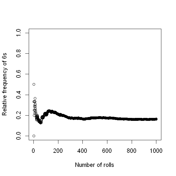
One way to define probability is through the notion of relative frequency. If we carry out an experiment (e.g. rolling of a die) a large number of times, then the proportion of times a particular result (e.g. a six) occurs is known as the relative frequency. If we repeat the experiment a very large number of times then the limiting value of the relative frequency (i.e. the value that the relative frequency approaches as the number of times approaches infinity) is called a probability.
The plot below shows the relative frequency of 6s when a die is rolled repeatedly. The first roll was not a 6, and so the relative frequency is zero. The second roll was a 6, so the relative frequency is 0.5. As we then roll the die further, the relative frequency fluctuates. But from the figure we see that as the number of rolls increases, the relative frequency converges to 1/6.
set.seed(123)
roll <-sample(1:6,1000,replace=T)
n <- seq_along(roll)
d <- cumsum(roll==6)/n

options(repr.plot.height=5, repr.plot.width=5)
plot(n, d,
  xlab="Number of rolls", ylab="Relative frequency of 6s",
  xlim=c(1, 1000), ylim=c(0, 1))
Probability is crucial to medical statistics. For example:
Predicting events
What is the probability that a particular patient will suffer from heart disease in the next 10 years?
Assessing whether two characteristics are related
Is Left-Ventricular Ejection Fraction (LVEF; a measure of how well a heart is functioning) related to systolic blood pressure?
Quantifying uncertainty around estimates
We estimate that this new drug decreases 10-year mortality by 5%. Can we provide a range of values which captures the uncertainty around this estimate?
Answering each of these questions requires the use of probability.
Defining events
An experiment is a process that produces one outcome from some set of alternatives.
The sample space is the set of points representing all the possible outcomes of an experiment. The sample space is often denoted by \(\Omega\).
An event is a subset of the sample space.
Example
One experiment might be as follows:
Randomly select an individual from a population.
Record that individual’s asthma and smoking status.
Suppose we let \(A\) denote the event that the selected individual has asthma (and therefore \(\bar{A}\) denotes the individual not having asthma). Similarly, let \(S\) denote the event that the selected individual is a smoker (\(\bar{S}\) denotes that the selected individual is not a smoker).
The sample space contains four elements:
One event of interest would be the event that the randomly selected individual is a smoker. This is the subset:
Venn diagrams and set notation
Venn Diagrams are sometimes used to represent probabilities in the whole sample space graphically. The whole diagram (bordered by the rectangle) represents the sample space and events within it are drawn with areas proportional to their probabilities. Note that sometimes, however, the areas are not drawn proportional to probability for aesthetic reasons!
The union of two events \(X\) and \(Y\), denote \(X \cup Y\), is the event that either \(X\) occurs, or \(Y\) occurs, or both occur. For example, \(A \cup S\) is the event that the randomly selected individual has asthma, is a smoker, or has asthma and is a smoker.
The intersection of two events \(X\) and \(Y\), denoted \(X \cap Y\), is the event that both \(X\) and \(Y\) occur. It is sometimes referred to as the joint probability of \(X\) and \(Y\). For example \(A \cap S\) is the event that the randomly selected individual has asthma and is a smoker.
The complement of an event \(X\), denoted \(\bar{X}\), is the event that \(X\) does not occur. The complement of \(X\) is also sometimes denoted \(X'\).
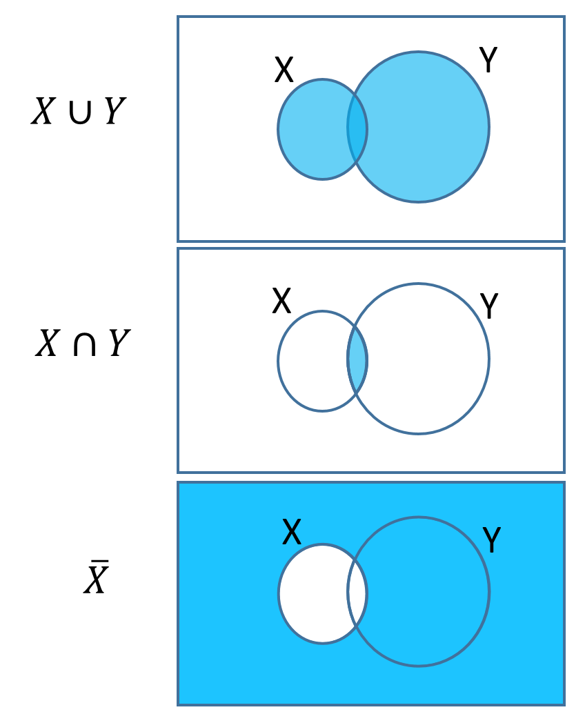
Fig. 1 Venn diagrams
Axioms of probability
We write \(P(A)\) to denote the probability of event \(A\) occurring.
The probabilities of events must follow the axioms of probability theory:
\(0 \leq P(A) \leq 1\) for every event \(A\).
\(P(\Omega)=1\) where \(\Omega\) is the total sample space.
For disjoint (mutually exclusive) events \(A_{1},..,A_{n}\):
The events \(A_{1},..,A_{n}\) are disjoint if at most one of them can occur, i.e. there are no intersections between any of the events.
Axiom 3 is sometimes referred to as the additive rule of probability.
Consequences of the axioms of probability
Given these axioms we can prove a number of useful results. Drawing a Venn diagram often helps us in constructing a proof, by appealing to a our visual intuition.
For example, using the axioms above, we can prove the complement rule:
We can similarly prove the useful rule for non-disjoint events \(A_1\) and \(A_2\),
Proof is left as an exercise.
Conditional probability
Suppose that we know that an individual is a smoker. Given that event, what is the probability that the individual suffers from asthma? This is known as a conditional probability.
We can write this as \(P(A|S)\). This is called the conditional probability of \(A\) given \(S\), i.e. the sample space is now reduced to \(S\) as we know the individual is a smoker. Once \(S\) has occurred, the event of interest will occur only if the observed outcome is in \(A \cap S\).
In the original sample space \(A \cap S\) has probability \(P(A \cap S)\) with denominator \(P(\Omega)=1\), but the conditioning has reduced the sample space, so the new probability is relative to this, i.e. \(P(A \cap S)\) as a portion of \(P(S)\). In the Venn diagram below, the sample space has been reduced to the non-grey parts due to the conditioning.
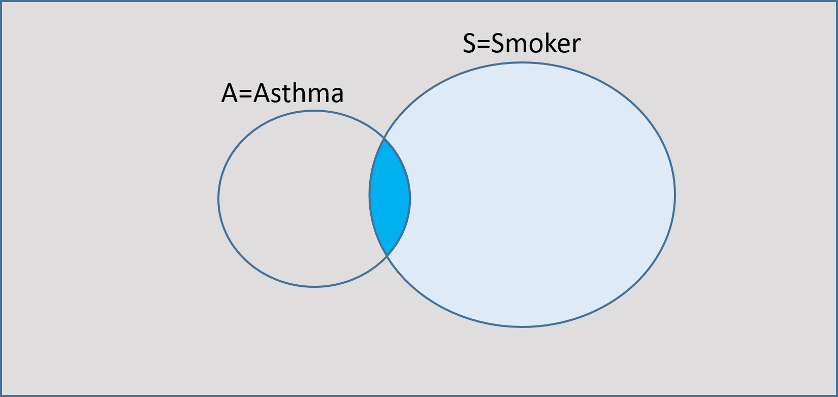
Fig. 2 Reduced sample space in conditional probability
This leads to the definition of conditional probability
Multiplying through by \(P(S)\), we see this implies that
This relationship is symmetric, so also:
Probability trees
A good way of displaying and calculating simple conditional probabilities is through the use of a probability tree. The different outcomes are represented by the different branches of the tree. The events in a probability tree are exhaustive (every possible event is accounted for) and mutually exclusive, so you must go along one branch and only one branch at each stage.
The simplest form of a probability tree is shown in the figure below. The second branches are all conditional probabilities, conditional on the events in each of the previous branches.
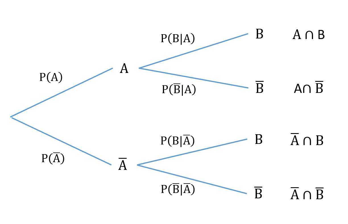
Fig. 3 Probability tree
To calculate the probability of taking a particular path through the tree, we multiply the probabilities of the corresponding branches. That this is correct is a consequence of our earlier result that
Example
Suppose we know that in the population of interest the prevalence of smoking is 20% among adults in general and that 9% of smokers suffer asthma whereas 7% of non-smokers have asthma. This information can be represented in a probability tree. Note that we are given \(P(A)\), \(P(A|S)\) and \(P(A|\bar{S})\), so the first branch of the tree is for smoking status and the second branch is asthma status conditional on smoking status.
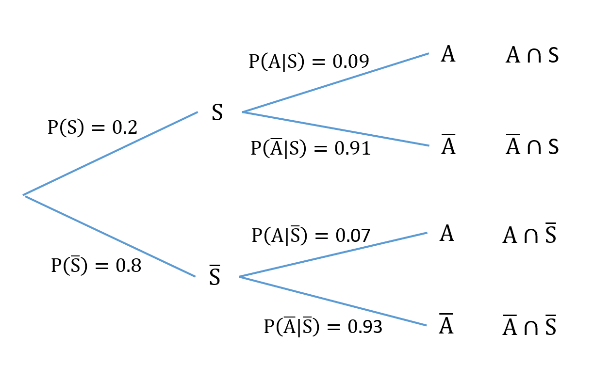
Fig. 4 Probability tree for the asthma example
The probability of any intersection of asthma and smoking events can then be obtained by multiplying the probabilities along the branches of the tree leading to the tip which corresponds to the desired event. For example
i.e. less than 2% of the population are both asthma sufferers and smokers.
Each tip of the tree represents an outcome of the “experiment”, and together the corresponding probabilities sum to 1.
Independence
A concept of fundamental importance in probability theory and medical statistics in particular is that of independence between events. Suppose that the occurrence of an event \(A_{1}\) provides no information at all about the probability of a second event \(A_{2}\) occurring (e.g. suppose that knowing someone was a smoker gave no information about whether or not they had asthma).
In that case, \(P(A_{2}|A_{1})=P(A_{2})\). i.e. knowing that \(A_{1}\) has occurred does not affect the probability that \(A_{2}\) will occur. Then
The latter is usually how independence between two events \(A_{1}\) and \(A_{2}\) is formally defined, i.e. \(A_{1}\) and \(A_{2}\) are said to be independent if
This is known as the multiplicative rule of probability.