Continuous Random Variables
A discrete random variable \(X\) takes values in a finite or countably infinite set, and is characterised by the probabilities \(P(X=x_{j})\) for the possible values \(x_{j}\) it might take. For example, e.g. \(X=\) weight measured to the nearest kg (for people who weigh between 50kg and 61kg) would be a discrete random variable.
Conversely, continuous random variables arise when a random variable takes values in an uncountably infinite set, such as the set of real numbers.
Probability density functions
For continuous random variables \(X\), the probability that \(X\) will take any particular value \(x\) is actually zero. This is because although \(X\) will take some value, there are so many possible values it could take the probability that it will take any particular value is zero. Instead of assigning probabilities to particular values, we define a probability density function \(f(x)\) (also sometimes abbreviated PDF) such that for any two values \(a\) and \(b\),
So the probability that \(X\) takes a value between \(a\) and \(b\) is equal to the area underneath the density function between \(x=a\) and \(x=b\).
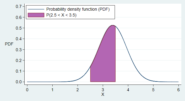
Fig. 5 A probability density function
Probability density functions must satisfy a number of conditions, which ensure that the axioms of probability are not violated:
\(f(x)\geq 0\) for all \(x\)
\(\int^{\infty}_{-\infty} f(x) dx = 1\)
This second condition is the continuous equivalent of the \(\sum_{x_{j}} P(X=x_{j}) = 1\) requirement for discrete random variables. Notice that it is possible for \(f(x)>1\), in contrast to the requirement for discrete \(X\) that \(0 \leq P(X=x_{j}) \leq 1\).
Cumulative distribution function
For continuous \(X\), the CDF is defined as:
which is the area under the curve (of the density function) to the left of \(x\). Note that when \(x\) appears in the bounds of the integral, we do not use \(x\) as the index within the integral (i.e. the integral contains \(f(t) dt\) and not \(f(x) dx\)).
Probabilities can be expressed using the CDF too:
Relationship between CDF and PDF
The CDF is the integral of the PDF (above). Therefore, we also have that
Expectation and variance of continuous random variables
Expectation is defined for continuous random variables \(X\) as for discrete \(X\), but with the summation replaced by an integral:
The variance is again defined as the expectation of the difference between \(X\) and its mean, squared: The variance of continuous \(X\) is thus given by:
As for discrete variables, we have the alternative form: \(Var(X) = E(X^2) - E(X)^2\).
Some rules for expectation and variance
The rules that we encountered for discrete variables also hold here. If \(a\) and \(b\) are constants, and \(X\) is a continuous random variable then:
\(E(aX + b) = aE(X) + b\)
\(Var (aX + b) = a^2Var (X)\)
For two continuous random variables, \(X\) and \(Y\), we have:
\(E(X + Y ) = E(X) + E(Y)\)
If \(X\) and \(Y\) are also independent then:
\(E(XY) = E(X)E(Y)\)
\(Var (X + Y) = Var (X) + Var (Y)\)
Expectation and variance of functions of a random variable
For a function of a random variable \(X\), \(g(X)\), we define the expectation as
And the variance is
Joint continuous distributions
Earlier, we introduced the concept of the joint probability distribution of two discrete random variables \(X\) and \(Y\). The idea extends naturally to the case of two continuous random variables \(X\) and \(Y\). For constants \(a, b, c\) and \(d\),
The joint density function must satisfy
and
The marginal distribution of one variable can be obtained from the joint density function:
The (joint) cumulative distribution function for \((X,Y)\) is defined by:
Although we will not go into the details further here, we can make corresponding definitions for the joint distribution of mixtures of continuous and discrete random variables.
Independence
Two continuous random variables \(X\) and \(Y\) are independent if their joint density function can be factorised into the product of their marginal densities, i.e.