Distributions
This page goes through some distributions that you may encounter during this year. This is to give a flavour of things to come; we do not expect you to know the details on this page when you start the programme.
This page can be read in a static format. Alternatively, open a local copy of R and copy each cell of code (by clicking the button at the top right of each code cell). Paste into your local R and run there.
Parameters
The word parameter refers to an unknown quantity. We often think about a parameter as being the “true” value, or the value that holds in a wider population of interest.
Most distributions have one or more unknown parameters which define the distribution.
Discrete distributions
Bernoulli distribution
The simplest discrete distribution that we are likely to encounter is the Bernoulli. The Bernoulli distribution corresponds to a single binary outcome (1=”success”, 0=”failure”), with \(P(X = 1) = \pi\).
If random variable \(X\) follows a Bernoulli distribution then we can write
where the \(\sim\) can be read as “follows the distribution of” or “is distributed as”. The expectation and variance of a variable \(X\) which follows a Bernoulli distribution with parameter \(\pi\) are given by:
\(E(X) = \pi\)
\(Var(X) = \pi(1-\pi)\)
So if we randomly generate a value for \(X\), it will either take the value of 0 or 1. If we do this many times (e.g. 50 times), then each of those 50 values will take the value either 0 or 1. The expectation - the long-run average - is \(\pi\). So if we simulate a large number of values, we expect the sample mean to be around \(\pi\). And we expect the sample variance to be around \(\pi(1-\pi)\).
The probability distribution function (PDF) of a Bernoulli variable is given by the single probability \(P(X = 1) = \pi\). This fully characterises the whole distribution since it determines \(P(X=0) = 1-\pi\).
The code below (in R) randomly generates values from a Bernoulli distribution. The first number is the number of values to draw (generate). We have set this to \(50\). This means that the object \(X\) contains \(50\) realisations from a Bernoulli distribution. So each of those 50 values will be a draw from \(Bernoulli(\pi)\). The second number is always 1 for a Bernoulli distribution. The third number is the probability of success, \(\pi\). Here, we have set \(\pi=0.3\). If you are reading this interactively, change the first and third number and see what happens to the individual values, sample mean and sample variance.
The command head(X) displays the first few values of the object \(X\) (i.e. it writes the first few values drawn for \(X\) on screen, in this case the first six values drawn for \(X\) were two zeros followed by a one and three more zeros). The mean(X) and var(X) commands display the sample mean and sample variance of \(X\).
X <- rbinom(50, 1, 0.3)
head(X)
mean(X)
var(X)
- 0
- 0
- 0
- 1
- 1
- 1
Binomial distribution
Now suppose we conduct many Bernoulli trials (we will call this number \(n\)) and combine the results together to form a single number - the total number of “successes” among the \(n\) trials. This number follows a binomial distribution.
Let \(X\) be the total number of successes from \(n\) trials. Then \(X\) follows a binomial distribution,
The expectation and variance of a variable \(X\) which follows a binomial distribution with parameter \(\pi\) and a fixed number of \(n\) trials, are given by:
\(E(X) = n \pi\)
\(Var(X) = n \pi(1-\pi)\)
The probability distribution function \(X\) is
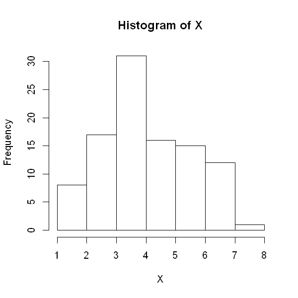
The code below randomly generates values from a binomial distribution. The first number is the number of values to draw (generate). If we set this number to 100, as below, then the object \(X\) will contain 100 different draws from a binomial distribution. The second number is the number of trials \(n\). The third number is the probability of success, \(\pi\) within each trial. If you are reading this interactively, change the first and third number and see what happens to the individual values, sample mean and sample variance.
X <- rbinom(100, 10, 0.48)
head(X)
options(repr.plot.height=5, repr.plot.width=5)
hist(X)
mean(X)
var(X)
- 3
- 4
- 2
- 5
- 4
- 5
Poisson distribution
The Poisson distribution is used to model the number of events occurring in a fixed time interval \(T\) when:
events occur randomly in time,
they occur at a constant rate \(\lambda\) per unit time,
they occur independently of each other.
A random variable \(X\) which follows a Poisson distribution can therefore take any non-negative integer value. Examples where the Poisson distribution might be appropriate include:
Emissions from a radioactive source,
The number of deaths in a large cohort of people over a year,
The number of car accidents occurring in a city over a year.
The parameter for the Poisson distribution is the expected number of events, \(\mu\). This can be calculated from the rate as \(\mu=\lambda T\). Often, the time period of interest is equal to one unit (in whatever units of time we are measuring in) in which case \(\mu=\lambda\).
If \(X\) is the total number of events occurring in a fixed interval \(T\) at a constant rate \(\lambda\) with parameter \(\mu=\lambda T\), then we write
The expectation and variance of a variable \(X\) which follows a Poisson distribution with parameter \(\mu\) are given by:
\(E(X) = \mu\)
\(Var(X) = \mu\)
The probability distribution function of \(X\) is
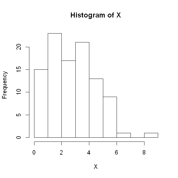
The code below randomly generates values from a Poisson distribution. The first number is the number of values to draw (generate). The second number is the number of trials \(n\). The third number is the probability of success, \(\pi\) within each trial. If you are reading this interactively, change the first and third number and see what happens to the individual values, sample mean and sample variance.
X <- rpois(100, 3)
head(X)
options(repr.plot.height=5, repr.plot.width=5)
hist(X)
mean(X)
var(X)
- 1
- 1
- 2
- 4
- 1
- 4
Hypergeometric distribution
In health settings, this distribution is perhaps less commonly used than the Bernoulli, binomial and Poisson.
When the population size \(N\) and number of successes in the population \(M\) are large, the variable \(X\) recording the number of successes in a sample of size \(n\) has a binomial distribution (see above). This approximate result fails when the population size \(N\) is small. Suppose then that we have a population of size \(N\), with \(M\) individuals having the characteristic corresponding to “success”, i.e. \(M\) out of \(N\) individuals in the population have a particular disease. We do not assume that \(N\) and \(M\) are large.
Let \(X\) be the random variable recording the number of individuals with the disease of interest in a sample of size \(n\) from a population of size \(N\), of which \(M\) individuals have the disease. Then \(X\) follows a hypergeometric distribution.
and
Continuous distributions
The normal (Gaussian) distribution
The normal (Gaussian) distribution is arguably the most important probability distribution in statistics. It lies at the heart of the modelling assumptions of linear regression and plays a critical role in statistical inference because of the Central Limit Theorem.
The normal distribution has a ‘bell-shape’. It is centred around its mean, \(\mu\). The spread of the different values is determined by the variance, \(\sigma^2\).
If a variable \(X\) follows a normal distribution, with parameters \(\mu\) and \(\sigma^2\), we write
The expectation and variance of a variable \(X\) which follows a normal distribution with parameters \(\mu\) and \(\sigma^2\) are given by:
\(E(X) = \mu\)
\(Var(X) = \sigma^2\)
The probability distribution function of \(X\) is
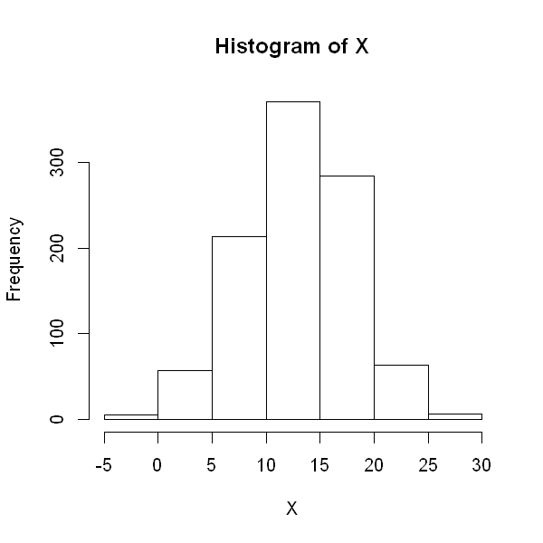
The code below randomly draws 1000 observations from a normal distribution. If you are reading these notes interactively, try changing the values \(\mu\) and \(\sigma^2\) in the first two lines and see how the histogram of values change.
If you would like to see the values generated, try adding the lines of code head(r) and summary(r).
mu <- 13
sigma2 <- 5
X <- rnorm(1000, mu, sigma2)
options(repr.plot.height=5, repr.plot.width=5)
hist(X)
The standard normal distribution
A special case of the normal distribution is the standard normal, which is a normal distribution with mean 0 and variance 1. We often use the letter \(Z\) to denote a variable that follows a standard normal distribution. For a standard normal variable, \(Z\), 95% of the distribution is contained between -1.96 and +1.96:
A useful property of normal distributions is that any normal distribution can be transformed to the standard normal distribution by subtracting the mean and dividing through by the standard deviation (the square root of the variance). So if
then
One consequence of this is that for any normal distribution, 95% of the observations are contained within \(\pm 1.96 \sigma\) of the mean \(\mu\).
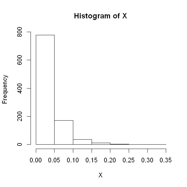
The exponential distribution
Suppose the number of events in a period follow a Poisson distribution and occur at rate \(\lambda\), with \(\lambda>0\). Consider the time between two consecutive events. The distribution of this variable is called the exponential.
If a variable \(X\) follows an exponential distribution, with parameter \(\lambda\), we write
The expectation and variance of a variable \(X\) which follows an exponential distribution with parameter \(\lambda\) are given by:
\(E(X) = \frac{1}{\lambda}\)
\(Var(X) = \frac{1}{\lambda^2}\)
The probability distribution function of \(X\) is
rate <- 30
X <- rexp(1000, rate)
options(repr.plot.height=5, repr.plot.width=5)
hist(X)
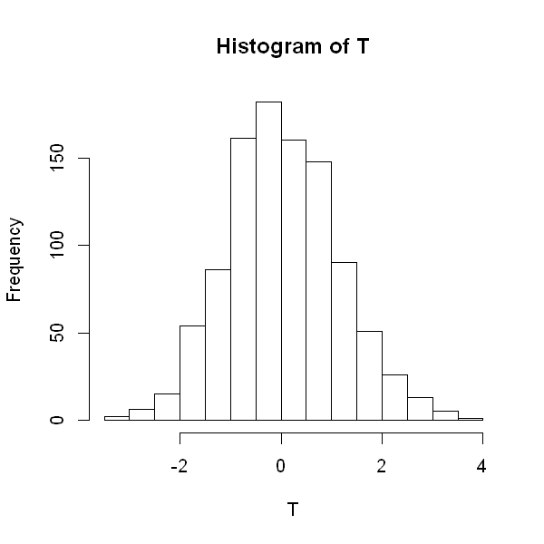
Student’s t-distribution
Student’s t-distribution arises as the ratio of the sample mean to its standard error. The t-distribution has a complex density function which we shall not state here. For now we note that the t-distribution has an additional parameter of sorts, known as the degrees of freedom (d.f.). The density function is similar to that of the standard normal, but the t-distribution has heavier tails. We often use \(T\) to denote a variable which follows a t-distribution. If \(T\) follows a t-distribution with \(\nu\) degrees of freedom, we write
The expectation and variance of a variable \(X\) which follows a t-distribution with \(\nu\) degrees of freedom are given by:
\(E(T) = 0\)
\(Var(T) = \frac{\nu}{\nu - 2}\) if \(\nu >2\); \(\infty\) for \(1<\nu \leq 2\); undefined otherwise
As the number of degrees of freedom increases the t-distribution gets closer and closer to the standard normal distribution. In the code below (if using interactively), try decreasing and increasing the degrees of freedom to see how the shape of the distribution changes.
df <- 18
T <- rt(1000, 18)
options(repr.plot.height=5, repr.plot.width=5)
hist(T)
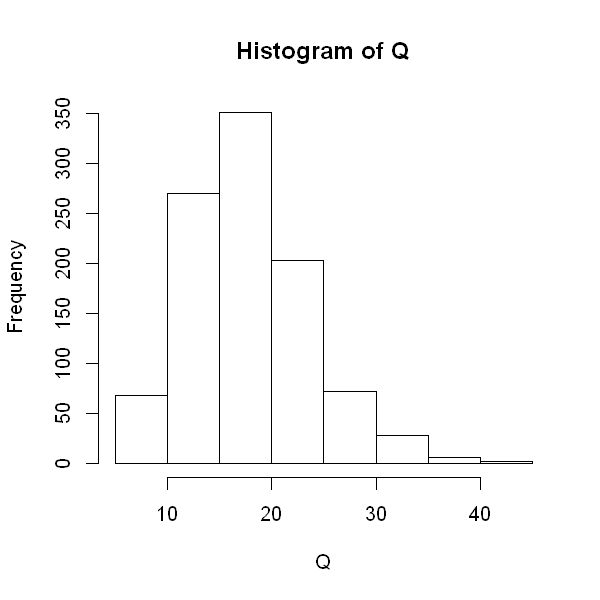
Chi-squared distribution
The chi-squared distribution with \(n\) degrees of freedom arises as the sum of the squares of \(n\) independent standard normal variables.
Thus if \(X_{1},..,X_{n} \sim N(0,1)\) and are independent and
Then \(Q\) follows a chi-squared distribution on \(n\) degrees of freedom. We write
The expectation and variance of \(Q\) are given by:
\(E(Q) = n\)
\(Var(Q) = 2 n\)
The probability distribution function is complex and not stated here.
The chi-squared distribution is used in a number of areas of statistics, such as when estimating the variance of a normal distribution, and in hypothesis testing to examine if there is evidence of an association between two categorical variables.
df <- 18
Q <- rchisq(1000, 18)
options(repr.plot.height=5, repr.plot.width=5)
hist(Q)
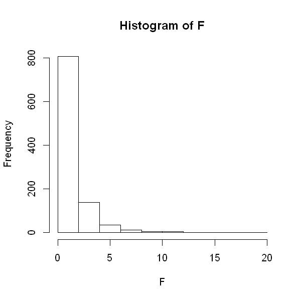
The F-distribution
The F distribution arises as the ratio of two independent chi-squared distributions.
Suppose \(U_{1} \sim \chi^{2}_{n}\), \(U_{2} \sim \chi^{2}_{m}\) and \(U_{1},U_{2}\) are independent, then:
We write \(F \sim F_{n,m}\).
The F-distribution arises when performing hypothesis tests in an analysis of variance and linear regression.
df1 <- 4
df2 <- 9
U1 <- rchisq(1000, df1)
U2 <- rchisq(1000, df2)
F <-(U1/df1)/(U2/df2)
options(repr.plot.height=5, repr.plot.width=5)
hist(F)
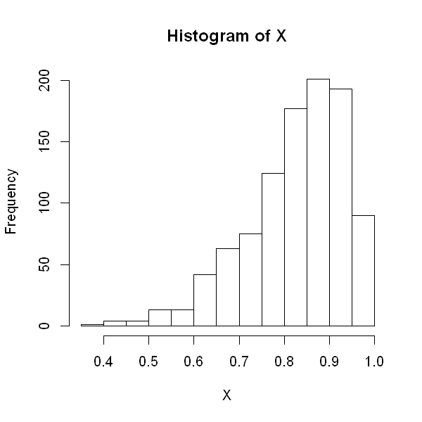
The Beta distribution
The beta distribution is a continuous probability distribution with two parameters, often called shape parameters since they control the shape of the distribution. If \(X\) follows a Beta distribution, we write
The density of the Beta distribution is:
The Beta function, \(B(\alpha, \beta)\) is a normalisation constant to ensure that the integral from 0 to 1 is equal to 1.
The Beta distribution appears frequently in Bayesian inference. It can also be used to model percentages and proportions. The expectation and variance is given by:
\(E(X) = \frac{\alpha}{\alpha + \beta}\)
\(Var(X) = \frac{\alpha \beta}{(\alpha + \beta)^2 (\alpha + \beta + 1)}\)
alpha <- 10
beta <- 2

X <- rbeta(1000, alpha, beta, ncp = 0)
options(repr.plot.height=5, repr.plot.width=5)
hist(X)