1 Introduction
Statistics for Health Data Science is the scientific approach behind investigating health. The organisers of this module have been specific in the wording. Of course, we will learn techniques to interogate data using statistics! But also, the focus on the approach is to think about a problem scientifically, for example to consider a research question, or a hypothesis. The scientific approach is important, and is described in more detail in this Introduction and the associated lecture. The scientific inquiry is applied to health data, which can take a number of forms, including ‘found data’. We think this is what makes data science for health unique; found data presents great advantages as there may be a lot of found data avaialble, but also challenges as the origin of the data and the potential for biases in the data can make analysis more challenging.
consider the concept of Statistics for Health Data Science and the bigger picture of scientific inquiry
understand the data by identifying broad issues of structure, type, provenance and design
describe variable types
understand the concept of selection bias
think about data summaries using exploratory data analysis and visualizations (simple examples)
consider what to measure and why in a scientific study
have a basic understanding of the difference between frequentist (Fisher) and Bayesian inference
1.1 What you will learn
By engaging with module you will acquire skills that a data scientist will need to interogate data to answer a health related question. Much of the focus is on the statistical tools that are most often used, as shown above in the Intended Learning Objectives. The module is designed towards using statistics within a problem solving cycle (more in Section 1.3).
Consider this book to be a practical guide in using statistics. Every session provides some statistical theory and examples so you can see the theory in action. Especially in the earlier sessions, some of the examples can be done without using a computer. As the module progresses many of the calculations are carried out using R, and we will increasingly apply the concepts to real data. We provide the code for each example.
As you work through the sessions, your ability to use statistics in health data science should improve. We will begin with relatively simple questions that we want to answer. As the module progresses, the questions will be more relevant to a health, and the steps involved will require more statistical inference and scientific inquiry.
Module layout
The module is roughly divided into three sections: Basic Probability, Statistical inference and Statistical modelling. Each sections build upon the previous. Probability is perhaps an obvious underpinning of statistics; it gives us the building blocks for both statistical inference and modelling. In probability (sessions 2 and 3) we cover discrete and continuous distributions, and make use of the maths refresher in several sessions. Fundamentally, when dealing with data we often need to make assumptions about what distribution the data is drawn from, and knowing the properties of these distributions then enables us to carry out statistical inference. When we move to statistical inference (sessions 4 to 10) this gives us the understanding of how statistical theory can be used to make statements during our investigations. An important consideration is thinking about the statistical theory that enables us to invesitgate our data, but then use this knowledge to then make statements about the wider population (or target population). With this knowledge we then move to Bayesian statistics, where we apply our knowledge to specific health questions and make use of prior knowledge. We then move onto applications that are more likely to be encountered in health applications; and consider the process of investigation and statistical modelling (sessions 11 to 17). These sessions are linked together because as well as being able to run a model and generate results, it is very important to articulate why it was done, ie. identify the purpose of investigation. In the sessions on regression modelling several classes of model will be described and illustrated in detail.
At the end of the module there will be a revision session, and an assessment (more detail is provided on Moodle).
1.2 What you won’t learn
We provide important aspects of statistical theory in order for you to understand the reasoning behind the approaches, but there are aspects of statistical theory that are outside of the module scope. In this case, we may provide further reading. Other modules within the LSHTM may cover this in more detail, such as Foundations of Medical Statistics.
This module provides the basics that further modules in the MSc may require, such as Data Challege and Machine Learning. As the name might imply, the statistical techniques used in machine learning are covered in the other module.
The programming associated with this module is carried out in R. The statistical analysis can be carried out in other software, such as Python. In some of the later sessions, we will provide the equivalent Python code, but we do not expect you to use this (and you will not be assessed on this).
1.3 The Data Science Project
Once a health related question is posed, this could be the start of a Data Science Project. Typically, we try to frame the question around a scientific hypothesis, identify some data that can be used to address this question/hypothesis, carry out some anlaysis and draw a conclusion. In David Spiegelhalter’s Book The Art of Statistics this process is referred to as the PPDAC cycle (fig. 1.1). If doing data science is new to you, this might be considered a linear process. But, in many circumstances the problem solving process is a cycle, where a problem may be solved using a iterative process. The iterative process doesn’t mean that the first attempt was wrong, but instead this iterative way of thinking enables the data scientist to think critically about each stage of the cycle and identify strengths, weaknesses and opportunities for improvement.
Note that there are many ways to describe the cycle of a Data Science Project, and more examples are given in the lecture by Prof. Nick Jewell. Some might chime with you more (or less) than the PPDAC presented here.
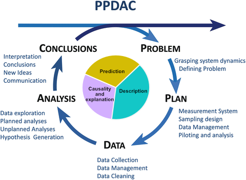
Fig. 1.1 The PPDAC cycle (From The Art of Statistics by David Spiegelhalter)
1.3.1 Identify the problem and generate a hypothesis
Typically Health Data Science projects start with a question. The question may be framed around one of three investigation types: description, prediction and causality and explanation. The specific of this is explored in more detail in Session 11 (Types of Investigation).
When developing a Data Science Project there is a need to create a question that is answerable within the timeframe available, and sufficiently precise. It is also preferable to frame a question around a hypothesis that can be a testable prediction, and this is where statistics can be used, because a lot of statistics are framed using a hypothesis (this is especialy true of frequentist statistics). However, it is not always necessary to have a hypothesis, for example if the question is exploratory.
1.3.2 Develop a plan, consider the data design
The plan to answer the question/hypothesis will involve some data. For data science it is likely that the data has not been collected specifically for the purposes of answering the question. Examples may include surveillance data for infectious diseases (eg. self-reported cases of influenza-like illness to a public website) or internet searches for “sore throat”. In this case, it is important to recognise specific attributes of the data:
Where did the data come from? What is its provenance?
How and why was the data collected?
What kind of individuals provided data, and why were they selected?
These are important questions because they relate to the principles of statistical inference, which is covered in sessions 4-10. Central to using data to draw a conclusion is that your sample data is representive of the population. Consequently, we can carry out an analysis on the data and make statements about the wider population. This is covered in more detail in session 4 (Populations and Samples).
At this stage it is important to identify the “outcome” variable and the “explanatory variables” present in the dataset, and whether we know already that some explanatory variables are associated with the outcome variable. It is also a good idea to idenitfy what type of data each variable corresponds to: continuous, ordinal, categorical.
The design of the dataset is also important, as this helps us understand the structure of the data, and a framework for analyses on the data. Commonly encountered designs are (note that these are also covered in the Epidemiology for Health Data Science module):
A cross-sectional design
A cohort design
An outcome-based design
A longitudinal design
At this stage, you may start to consider the appropriate analysis to make considering the data. As the module (and others, for example the Data Challenge module) develops you will identify the analysis steps that can be undertaken according to the question.
1.3.3 The data
There are several aspects of the data that need to be considered, and some of which are covered in the module Health Data Management, such as entering the data, managing the data, and cleaning the data.
Here we will focus on aspects which might affect the analysis and conclusions that you make later in the PPDAC cycle.
The first is the presence of potential data filtering, ie. is there any reason to suspect that data are missing or censored, in reference to to wider population? If so, this could result in potential bias. The most commonly encountered bias is selection bias, where extrapolation to the wider population may be challenging. Additionally, collider bias may result in inappropriate conclusions being made on the effect of explanaotry variables on the outcome.
The second consideration is confounding, where there may be a common cause for both a explanatory variable and the outcome. The result is that an assoication between the explanatory variable and the outcome may be identified, but the relationship is not causal.
1.3.4 Data analysis
Exploratory data anlaysis, and especially plotting your data is a really important part of the Data Science Project. As you progress through the module, this will become more and more familiar. Plotting your data is important to sense check the data and identify any errors, outliers or omissions (this is especially important with found data). Further to this, many statistical anlaysis benefit from plotting the results, for example by plotting the residuals of a linear model against the outcome to check that the model is correctly specified. Often, suitable plots may carry with them parameter estimates from the data, for example the mean number of influenza-like illnesses reported per week when the data are available daily.
It is at this stage that you do the analysis. This is where the concepts covered in this statistics module become useful. What we want to emphasize here is that this is done while considering all the others factors within the PPDAC cycle.
1.3.5 Conclusions
So you’ve gotten this far! An ideal conclusion has brought all the other aspects together, and at most stages some form of statistical inference is considered. The conclusion then needs to consider the statistical result in the context of the other considerations, such as wanting to make inference about the population from the sample of data.
For example, let’s say the influenza-like illness data from the internet reported 40 cases per 100,000 of the population from November to January. Reporting symptoms might be skewed towards people who regularly use the internet, which might exclude elderly individuals. Consequently, this mean estimate may be an under-estimate of the population incidence due to selection bias.
1.6 Why we teach both frequentist and Bayesian statistics
A majority of the module covers statistical inference from the frequentist perspective. Much of frequentist statistical inference was developed by Ronald Fisher, who has been described as the founder of modern statistics, and much of his focus was on experimental design in agriculture. A simple explanation of the philosophy behind frequentist statistics is that a fact is either true or not true, and data can be used to assess which of these outcomes can be accepted. In contrast, Bayesian statistics suggests that a probability can be assigned to whether the fact is true. The field of Bayesian statistics is named after Reverend Thomas Bayes, who developed the theory almost 200 years before Fisher was alive (and owing to improvements in computation the theory is now much more accessible and has overtaken frequentist approaches in some scientific fields). In addition, frequentist statistics makes use of the data available, and there is little (or any) ability to incorporate additional knowledge. Within a Bayesian framework, inclusion of prior knowledge is inherent, and this prior knowledge can be combined with data.
Some argue that the philosophies are diametrically opposed to each other, and statisticians should choose a side. This is a strong view (and perhaps not the majority view?), but first it is important to understand the principles behind each approach. We have opted to teach both because of this reason, and leave it up to you to consider the advantages and disadvantages of each approach. Ultimately, both have data central to the approach in making statistical inference, so it is likely that both should be considered as perspectives in a Data Science Project.