11.5 Role of explanatory variables in different types of investigation
The role of explanatory variables in different types of investigation differs. We focus here on prediction investigations and causal investigations.
11.5.1 Prediction
In prediction investigations the aim is to use \(X_{1}\), … , \(X_{p}\) to predict \(Y\) . In this setting the \(X_{1}\), … , \(X_{p}\) are often referred to as the ‘predictors’ for obvious reasons. For a prediction problem we may well use all of the explanatory variables \(X_{1}\), … , \(X_{p}\) in the prediction model or algorithm. Crucially, in prediction we are not interested in the inter-relationships between the explanatory variables \(X_{1}\), … , \(X_{p}\) and their temporal ordering. The only aim is to achieve a good prediction of the outcome \(Y\). It may be desirable to reduce the number of explanatory variables, particularly in settings where the number of potential predictors \(p\) is very large. Various principled procedures are available for reducing the number of predictor variables.
11.5.2 Causality and explanation
In investigations of causality, one of the explanatory variables is designated as the treatment or exposure of interest. Let’s suppose this is variable \(X_{1}\) and the research question is about how \(X_{1}\) affects \(Y\). Or, in other words, if \(X_{1}\) had been different, how would \(Y\) have been different? Let’s consider the setting of an Randomized Controlled Trials and an observational study separately and think of the situation where \(X_{1}\) is a binary treatment variable
Randomized controlled trials (RCT)
Suppose individuals are randomized to receive treatment \((X_{1} = 1)\) or not \((X_{1} = 0)\), and the outcome \(Y\) is observed after some period of follow-up. It is straightforward to estimate the treatment effect in this setting because of the randomization. For a continuous outcome, we would quantify the treatment effect using a difference in the mean outcome in the two treatment groups \((E(Y |X_{1} = 1) − E(Y |X_{1} = 0))\). For a binary outcome we could quantify the treatment effect in terms of a risk difference \((Pr(Y = 1|X_{1} = 1) − Pr(Y = 1|X_{1} = 0))\), risk ratio \((Pr(Y = 1|X_{1} = 1)/Pr(Y = 1|X_{1} = 0))\) or odds ratio \(((Pr(Y = 1|X_{1} = 1)/Pr(Y = 0|X_{1} = 1))/(Pr(Y = 1|X_{1} = 0)/Pr(Y = 0|X_{1} = 0)))\), for example.
Some of the other explanatory variables \(X_{2}\), … , \(X_{p}\) are likely to be associated with \(Y\), but we do not need to use them to estimate the treatment effect due to the study design. Sometimes investigators will adjust for baseline variables, measured at the start of the trial prior to treatment. By the study design, baseline variables are not associated with the treatment. There can be advantages of adjusting for baseline variables that are predictors of the outcome. Though there are particular nuances to the interpretation of the resulting estimates depending on the types of outcome (continuous, binary, etc) and on how the treatment effect is quantified.
Of course, there are many important considerations surrounding the validity and interpretation of treatment effects estimated using RCTs, such as whether the effect is a ‘per-protocol’ or ‘intentionto-treat’ effect, whether there is drop-out, non-adherence or treatment switching.
Observational studies
Suppose we have available observational data on the treatment variable \(X_{1}\) and the outcome \(Y\), for example from electronic health records. In this setting the treatment in non-randomized, and there are very likely to be confounders of the association between the treatment and the outcome.
A confounder is a variable that affects both the treatment and the outcome. Confounding variables occur prior in time to both the treatment/exposure and the outcome. See VanderWeele and Schpitser (2013) for a formal statistical discussion of confounding.
To estimate the causal effect of \(X_{1}\) on \(Y\) requires us to control for confounding. Consider a simple setting in which there is only one other variable at play, \(X_{2}\), which in the observational setting affects whether a person gets the treatment \(X_{1}\) and also affects their outcome \(Y\). For example, if \(X_{1}\) is a blood pressure-lowering medication and \(Y\) is blood pressure 1 year later, then \(X_{2}\) could be the person’s blood pressure at the time origin. The assumed relationships between the three variables \(X_{1}\), \(X_{2}\) and \(Y\) are illustrated in Figure 2 using directed acyclic graphs (DAGs), contrasting the relationships in an RCT and in an observational study.
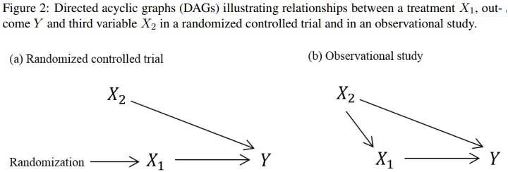
DAGs, also called ‘causal diagrams’, are used to graphically describe mechanistic relationships between variable using uni-directional arrows. An arrow connecting two variables indicates (potential) causation in the direction of the arrow and the absence of an arrow indicates an assumption that there is no direct causal effect of the first variable on the second. See Greenland et al. (Epidemiology, 1999) and Shrier and Platt (2008) for introductions to causal diagrams. Some other useful more recent articles on this are from Etminan et al. (2020) and Tenant et al. (2019). In simple situation such as this example, we don’t need a DAG to tell us that we need to account for the confounding by \(X_{2}\) in our analysis in order to estimate the effect of \(X_{1}\) on \(Y\) . However, when there are lots of variables at play DAGs become very useful, and have formal theory attached.
In summary, in a causal investigation the variables on which the research question focuses are \(X_{1}\) and \(Y\) . However, depending on the study design, we may need to account for other variables in the analysis, though those other variables are not our main focus. The concept of confounding is not relevant in prediction investigations.