4.3 Sampling distributions
In order to use our estimate (the value of the estimator in our sample of data) to make any sort of statement about the true but unknown value of the population parameter, we need to consider questions such as:
How precise do we believe our estimate is?
Are we fairly certain that the true parameter is close to the estimate, or do we believe the estimate may well be far from the true value?
The following thought experiment might help to develop these ideas. Suppose our population is a large bucket full of identical marbles. We want to know the population mean weight of a marble (our population parameter of interest). To estimate this population mean, we can simply sample a single marble from the bucket. So our estimator is the weight of the single sampled marble. Now suppose we took two samples: we sample a single marble, weigh it, put it back in the bucket, sample another marble and weight that one. In this case, our estimate (the weight of the sampled marble) would be exactly the same as the estimate from the first sample. No matter how many different samples we took, the sample estimate would be identical. In this case, because all possible samples would give us an identical estimate of the mean, we can confidently say what the population mean is using a single sample of one marble.
Now consider a bucket full of different marbles. In this case, randomly sampling a single marble and using the weight of that marble as an estimate of the population mean weight could give us a weight far too large (if we just happened to sample one of the very large marbles) or far too small (if we happened to pick a very small marble). However, if we were to pick 100 marbles and take the sample mean of those 100 marbles as our estimator, we would expect our estimate to be closer to the population mean. If we were to resample another 100 marbles we would expect the sample mean weight to be fairly close to the mean weight of the previous 100 marbles. Conversely, if we took two samples containing one marble each, we might expect those two weights to be quite different from one-another.
This thought experiment makes it clear that in order to use our single sample of data to make statements about a wider population, we need to think about what would happen if we repeated our sampling: if we re-did our study many times, each time calculating the sample estimate, what values would those different sample estimates take? In fact, this is exactly what the sampling distribution is. It is the distribution of the estimator (the statistic we have chosen to use to estimate the population parameter of interest) under repeated sampling.
4.3.2 Simulated data: sampling distribution of a mean
We will return again to the emotional distress study. In reality, we do not know the true population mean and standard deviation. However, for the purposes of illustration, for the rest of the session we will imagine that we do know these values. Suppose that, in truth, the population mean age (\(\mu\)) is 30 and the population standard deviation (which will will call \(\sigma\)) is 4.8. Further, suppose that age follows a normal distribution in the population.
Under this scenario, the following code draws many (10,000) different samples from this population, with each sample containing the ages of 10 people. Note the line set.seed(1042) is coded to keep the same pseudo random number starting point.
# Population parameters
mu <- 30
sd <- 4.8
n_in_each_study <- 10

# Draw samples and ages for sampled individuals, for 100 different studies
# in this example we're going to have a list which generates study_measurements_age repeatedly
different_studies <- 10000
set.seed(1042)
study_measurements_age <- list()
for (i in 1:different_studies) {
  study_measurements_age[[i]] <- round(rnorm(n_in_each_study, mu, sd),3)
}

# Print the sample data for two of the studies
print("Ages of the 10 participants selected in study 1:")
study_measurements_age[[1]]

print("Ages of the 10 participants selected in study 5:")
study_measurements_age[[5]]
[1] "Ages of the 10 participants selected in study 1:"
- 17.897
- 30.27
- 26.896
- 35.448
- 28.514
- 33.891
- 42.021
- 25.994
- 31.061
- 28.756
[1] "Ages of the 10 participants selected in study 5:"
- 28.502
- 33.725
- 35.155
- 26.544
- 31.147
- 31.732
- 39.582
- 31.223
- 25.802
- 16.168
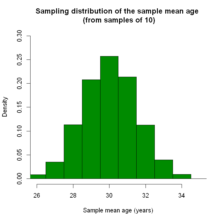
Now we will calculate the sample mean for each sample of 10 people and plot them on a histogram. In the graphs below, we see a graph of sample means from 10,000 different studies (i.e. 10,000 different samples). This only gives us an approximation to the true sampling distribution, because it is based on a finite number of samples (10,000 samples). However, this is a large number so it will give us a fairly good approxiation to the sampling distribution of the sample mean.
For this estimator and this population, we can see that the sampling distribution follows a normal distribution. Note that the sampling distribution is centred around the true population value of 30. We also see that almost all sample means lie within 4 or so years of the mean either way (i.e. most sample means are between 26 and 34).
options(repr.plot.width=6, repr.plot.height=6)
sample.means   <- sapply(study_measurements_age, mean)

# Draw graphs using base R
hist(sample.means[1:10000], freq=FALSE,
     breaks=c(0, 25.5, 26.5, 27.5, 28.5, 29.5, 30.5, 31.5, 32.5, 33.5, 34.5, 100),
     xlim=c(26, 35), ylim=c(0, 0.3), col="green4",
     xlab="Sample mean age (years)",
     main="Sampling distribution of the sample mean age \n (from samples of 10)")
4.3.3 The standard error of an estimate
When we are talking about the sampling distribution (i.e. the distribution of an estimator), we call the standard deviation the standard error. The standard error refers to the variability we might expect in estimates of the parameter, because we are inferring the estimates from a sample. When we have two different estimators for the population parameter of interest, we would typically choose the one with the lower standard error.
If an independently distributed random variable \(X\) has population mean (\(\mu\)) and population variance (\(\sigma^2\)), the sampling distribution of sample means (of samples of size \(n\)) has population mean \(\mu\) and population variance \(\sigma^2/n\). This irrespective of the population distribution; it does not need to be normal. In other words the standard error is \(\sigma_{\bar{X}} = \sigma/\sqrt{n}\).