10.3 Credible Intervals
We saw in the previous session that a Bayesian \(95\%\) credible interval is an interval which contains \(95\% \) of the posterior distribution of the parameter, and the \(95 \%\) Highest Posterior Density (HPD) interval is the credible interval with the smallest range of values for \(\theta\).
Given that the posterior distribution has mean \(\psi\) and variance \(\gamma^{2}\), the \(95\%\) HPD interval is given by \(\psi \pm 1.96 \times \gamma\). Thus, for a standard Normal posterior, the 95% HPD interval is \((-1.96,1.96).\)
10.3.1 CD4 cell counts example:
In the CD4 cell count example, suppose that we have very strong prior information that suggests the treatment is not effective, and we expect that the difference in cell counts is approximately zero. Let us denote by \(y\) the difference in CD4 cell counts. We set \(\mu \sim N(0, 0.1)\) to reflect that there is only about \(2.5\%\) chance that the treatment increases mean CD4 counts by more than 0.62 (1.96 \(\times \sqrt{0.1}\)) and a \(50\%\) chance that it will actually decrease the mean CD4 count).
Summarizing the information we have:
sample size \(n = 20\)
mean of data \(\bar{y} = 0.805\)
variance of data (assumed known) \(\sigma^2 = 0.7\)
prior mean \( \phi = 0\)
prior variance \(\tau^2= 0.1\)
We find the posterior distribution:
We plot below the prior distribution (in blue), the distribution of \(\bar{y}\) (red) and the posterior distribution (purple). We observe that the mean of the posterior distribution is in between the mean of the prior and that of the likelihood. Note that in R, the Normal distribution is parameterized by the standard deviation rather than the variance.
options(repr.plot.width=7, repr.plot.height=5)
x <- seq(-2, 2, 0.01)
#plot the prior
y1 <- dnorm(x, mean=0, sd=sqrt(0.1))
plot(x, y1, type="l", lwd=1, col="blue", ylim=c(0,3), ylab="Density", xlab=expression(mu))
legend("topleft", legend=c("Prior distribution", "Distribution of mean of y", "Posterior distribution"),
       col=c("blue", "red", "purple"), lty=1)
#plot the observed distribution
y2 <- dnorm(x, mean=0.805, sd=sqrt(0.7/20))
lines(x, y2, type="l", lwd=1, col="red")
y3 <- dnorm(x, mean=0.596, sd=sqrt(0.0259))
lines(x, y3, type="l", lwd=1, col="purple")
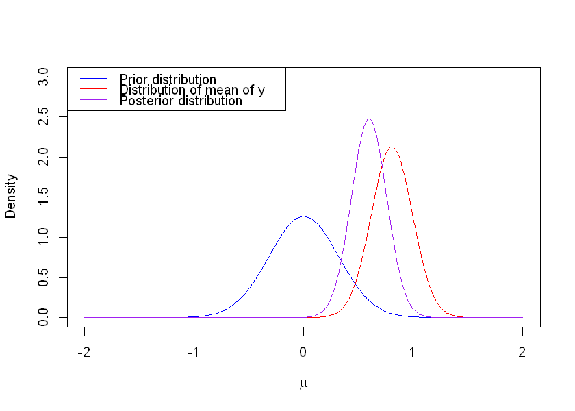
The \(95\%\) HPD interval can be calculated as \(0.596 \pm 1.96 \times \sqrt{0.0259} = (0.281, 0.911)\). This interval lies wholly above zero, so we can state that we have a strong posterior belief that there is an increase in CD4 cell counts.