12.2 Data used in our examples
For our examples we will use data on babies and their mothers. The data contains a random sample of 1,174 mothers and their newborn babies. The column Birth Weight contains the birth weight of the baby, in ounces; Gestational Days is the number of gestational days, that is, the number of days the baby was in the womb. There is also data on maternal age, maternal height, maternal pregnancy weight, and whether or not the mother was a smoker.
The following code can be used to download and look at the data:
#Load data
data<- read.csv('https://www.inferentialthinking.com/data/baby.csv')

#Look at the first 10 rows of the data
head(data)
| Birth.Weight | Gestational.Days | Maternal.Age | Maternal.Height | Maternal.Pregnancy.Weight | Maternal.Smoker |
|---|---|---|---|---|---|
| 120 | 284 | 27 | 62 | 100 | False |
| 113 | 282 | 33 | 64 | 135 | False |
| 128 | 279 | 28 | 64 | 115 | True |
| 108 | 282 | 23 | 67 | 125 | True |
| 136 | 286 | 25 | 62 | 93 | False |
| 138 | 244 | 33 | 62 | 178 | False |
12.2.1 Exploratory analyses
The simple linear regression model is used to model the relationship between one single variable (\(X\)) and a single outcome (\(Y\)). For example, suppose we are interested in investigating the following relationships in our birthweight data:
Association between the length of pregnancy (i.e. number of gestational days) and birthweight.
Association between mother’s smoking status and birthweight.
An important first step in an analysis is to summarise and display the data. Below is a scatterplot and boxplot displaying the relevant data for Examples 1 and 2 respectively.
data<- read.csv('https://www.inferentialthinking.com/data/baby.csv')

# Set the plot area into a 1x2 array
par(mfrow=c(1,2))
options(repr.plot.height=5)

# Example 1: Scatter Plot
plot(data$Gestational.Days, data$Birth.Weight, main="Example 1",
     xlab="Gestational Days", ylab="Birthweight (oz)", pch=19)

# Example 2: Box plot
boxplot(data$Birth.Weight~data$Maternal.Smoker, main="Example 2", xlab="Mother smokes", ylab="Birthweight (oz)")
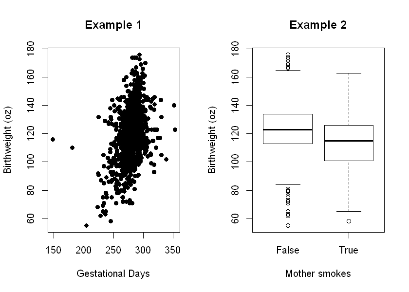
Example 1: Birthweight and gestational days appear to be highly correlated, where an increase in gestational days is associated with increased birthweight.
Example 2: It appears that mothers who do not smoke give birth to heavier babies, on average, than mothers who do smoke.
12.2.2 Determining the dependent and independent variables
Before defining a regression model, we have to decide which is the independent variable and which is the outcome (i.e. the dependent variable). In this context, it is natural to consider birthweight as the outcome: conceptually, it makes little sense to investigate how birthweight influences length of pregnancy or the mother’s smoking status. However, it is not necessarily always as straightforward. Suppose we were investigating the association between age and weight. It is possible that we might be interested in age as a predictor of weight, or in weight as a predictor of age. The aim of the analysis will guide the choice of outcome.
While the outcome is the same in our two examples, an important difference is the type of independent variable. In Example 1, the independent variable (length of pregnancy) is a continuous variable, whereas in Example 2, the independent variable (mother’s smoking status) is binary (yes or no). Using these examples, we will later see how the two different types of variables are modelled differently in linear regression.