7.5 Confidence Intervals using resampling
We saw that we can often create an approximate sampling distribution by resampling from our sample data. This is particularly useful in situations where there is no algebraic derivation for the sampling distribution.
We have seen that the important connection between sampling distributions and confidence intervals. So we would intuitively expect to be able to construct a confidence interval from the approximate sampling distribution we obtained using resampling. This is indeed possible. There are many ways of doing this, but the simplest and most intuitive method is the bootstrap percentile confidence interval.
The basic idea is very simple. We construct an approximate sampling distribution using bootstrap samples, as we did previously. Then we take the 2.5th and 97.5th percentiles of that distribution (the value such that 2.5% of the observations - the estimates across bootstrap samples - lie below the value; and the value such that 2.5% of observations lie above the value, respectively). These form the limits of our 95% confidence interval.
set.seed(78234)

# Read in the sample of 10 ages
ages <- c(28.1,27.5,25,29.9,29.7,29.9,39.9,33.6,21.3,30.8)

# Draw bootstrap samples
bootstrap_samples <- lapply(1:1039, function(i) sample(ages, replace = T))

# Calculate sample means in each bootstrap sample
r.mean <- sapply(bootstrap_samples, mean)

# Obtain the 2.5th and 97.5th percentiles of the sample means across bootstrap samples
(q<-quantile(r.mean, c(0.025, 0.975)))

# Draw the approximate sampling distribution with the percentile confidence limits marked in red
options(repr.plot.width=4.5, repr.plot.height=4.5)
hist(r.mean, freq=FALSE, main="Sampling distribution for mean \n with percentile 95% confidence limits", xlab="Sample mean")
abline(v=q, col="red")
- 2.5%
- 26.798
- 97.5%
- 32.501
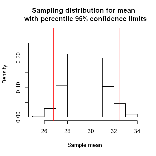
The approximate 95% confidence interval for the mean age obtained by using the algebric approximation to the sampling distribution was: 26.6 to 32.5. The bootstrap percentile 95% confidence interval is: 26.8 to 32.5. We see that these intervals are very similar to one another, as we would expect.