4.4 Obtaining the sampling distribution¶

The sampling distribution is hypothetical: in reality, we are not going to repeat our study many times to see how much our estimates differ from sample to sample.

In many cases we can describe the sampling distribution of our estimator well enough to do statistical inference, i.e. well enough to make useful statements about the population parameter. There are three main approaches to obtaining the (approximate) sampling distribution of an estimator:

Algebraic calculation. Sometimes we can algebraically obtain the distribution of the estimator from our statistical model. An example is given below for the sampling distribution for the sample mean age in the emotional distress example.
The Central Limit Theorem. If we have an estimator which can be written as the sum of independent random variables, then for large samples, the estimator will have an approximately normal distribution. This is described in more detail shortly.
Resampling. In many situations, we can use a resampling principle to obtain an approximate sampling distribution.

Returning to the question posed at the start of the previous section, those questions can be answered using the sampling distribution:

How precise do we believe our estimate is?

Are we fairly certain that the true parameter is close to the estimate, or do we believe the estimate may well be far from the true value?

The first question asks whether the sampling distribution is centred at the right value (i.e. the population parameter being estimated). If it is, we say the estimator is unbiased. In the epidemiology module and earlier in this module, you have already come across how the sample can be biased. Here, we are referring to whether the estimator is biased, which is sometimes referred to as statistical bias. Most estimators are unbiased, and this can be shown using statistical theory. For a small number of estimators it can be shown that they are in fact biased, and sometimes a correction can be applied to account for this. An example of exploring whether estimators are biased is given in the Appendix.

The second question will be examined when looking at the standard error and forms the basis for constructing 95% confidence intervals.

4.4.1 Algebraic calculation¶

We will illustrate the idea of obtaining a sampling distribution via algebraic calculation by revisiting the sub-sample from the emotional distress study.

For the moment, we will assume that in truth, ages follow a normal distribution with population mean \(\mu=30\) and population standard deviation \(\sigma=4.8\). Of course, in real life we would not have this information.

We now imagine that the population value of \(\mu\) is unknown to the investigators undertaking the study; indeed, making inferences about \(\mu\) is the aim of the study. We further imagine the rather unrealistic (but simplifying) situation that the investigators know the true value of the population standard deviation, \(\sigma=4.8\).

Our model for the emotional distress study states that:

\[ X_i \overset{\small{iid}}{\sim} N(\mu, 4.8^2), \qquad i=1,2,...,10 \]

Under this statistical model, we want to know the distribution of our estimator for \(\mu\):

\[ \hat{\mu} = \frac{1}{10} \sum_{i=1}^n X_i \]

In this case, it’s quite easy to derive the sampling distribution algebraically. We use the following fact:

The mean of independent normally distributed variables also follows a normal distribution

It is then easy to calculate the expectation and variance of \(\hat{\mu}\) using techniques covered in the maths refresher. So we know that the sampling distribution of \(\hat{\mu}\) is:

\[ \hat{\mu} \sim N\left(\mu, 1.52^2 \right) \]

where the variance of this normal distribution was obtained as

\[ Var(\hat{\mu}) = \frac{1}{10^2} \times 10 \times Var(X_i) = \frac{4.8^2}{10}. \]

This gives us a lot of useful information about how the sampling distribution in relation to the unknown parameter \(\mu\):

It follows a normal distribution (has a symmetric bell-shape)
It is centred around the true (unknown) population value
The standard error of the sample mean (the standard deviation of the estimator) is \(1.52\).

In many situations, this sort of algebraic calculation is possible. If not, we often rely on the central limit theorem to obtain the approximate sampling distribution in large samples.

4.4.2 The Central Limit Theorem¶

The Central Limit Theorem (CLT) is a key concept in statistics and in estimation. When we use the mean from a sample to estimate a parameter, we already acknowledge that there will be some error around this estimate, as described above. The CLT takes this further;

The Central Limit Theorem

If a random variable \(X\) has population mean \(\mu\) and population variance \(\sigma^2\) the sample mean \(\bar{X}\), based on \(n\) observations, is approximately normally distributed with mean \(\mu\) and variance \(\sigma^2/n\), for sufficiently large \(n\).

So even for situations where \(X\) follows a distribution that is not even close to being normal (e.g. \(X\) might be Poisson, or Binomial, or some wacky distribution), for sufficiently large samples the mean will follow a normal distribution. An example where \(X\) is a binary variable is given in the Appendix to this session.

This theorem is hugely powerful. We will see that this allows us to conduct large-sample inference fairly easily on any type of data.

4.4.3 Resampling¶

An alternative approach, which is computationally intensive but very flexible, is to use a resampling approach.

For a population of interest, we want to estimate a parameter \(\theta\) using a sample \(S\) of \(n\) individuals (for our example \(n=10\)) from the population. We have an estimator \(\hat{\theta}\) from our sample \(S\). We want to know about the sampling distribution of the estimator \(\hat{\theta}\).

We discussed above the idea that we could obtain the sampling distribution by repeatedly sampling from the population and calculating our estimate in each sample. Then a histogram of those many estimates would give us (approximately) the sampling distribution. In practice, it is logistically impossible to repeat the study a large number of times. However, we can mimic this process by using resampling.

The basic idea is to pretend that the observed data are the population and repeatedly sample from the data to learn about the relationship between \(\hat{\theta}\) and the estimates obtained from the re-sampled data, which we will call \(\hat{\theta}^*\).

Suppose we sample with replacement from the sample \(S\) to obtain “sub-samples” also of size \(n\). These “sub-samples” are called bootstrap samples.

For example, suppose we have a sample \(S\) of size 10 (\(n=10\)):

\[ S = \{ x_1, x_2, x_3, x_4, x_5, x_6, x_7, x_8, x_9, x_{10} \} \]

And suppose our estimate is the sample mean,

\[ \hat{\theta} = \frac{(x_1 + x_2 + x_3 + x_4 + x_5 + x_6 + x_7 + x_8 + x_9 + x_{10})}{10} \]

Then a bootstrap sample might be:

\[ S^*_1 = \{x_{10}, x_3, x_2, x_8, x_6, x_2, x_4, x_1, x_8, x_1 \} \]

Another bootstrap sample could be:

\[ S^*_2 = \{ x_5, x_9, x_4, x_7, x_{10}, x_9, x_3, x_4, x_6, x_2 \} \]

In each bootstrap sample, we obtain a new estimate (the sample mean in the bootstrap sample):

\[ \hat{\theta}^*_1 = \frac{(x_{10} + x_3 + x_2 + x_8 + x_6 + x_2 + x_4 + x_1 + x_8 + x_1)}{10} \]

and

\[ \hat{\theta}^*_2 = \frac{(x_5 + x_9 + x_4 + x_7 + x_{10} + x_9 + x_3 + x_4 + x_6 + x_2)}{10} \]

We do this a very large number of times to obtain lots of estimates from different bootstrap samples. Then we can draw a histogram of these many bootstrap estimates to see the shape and dispersion of the distribution.

The bootstrap principle says that the distribution of \(\hat{\theta}\) given \(\theta\) (i.e. the sampling distribution) is approximated by the distribution of \(\hat{\theta}^*\) given \(\hat{\theta}\). For example, if we find that our values of \(\hat{\theta}^*\) are approximately normally distributed and centred around \(\hat{\theta}\) then the bootstrap principle tells us that \(\hat{\theta}\) follows a normal distribution centred around \(\theta\).

4.4.3.1 Example: resampling¶

We illustrate the idea of resampling using the sub-sample of the emotional distress study. Suppose our data - the 10 sampled ages - are the set: \(\{ 28.1, 27.5, 25, 29.9, 29.7, 29.9, 39.9, 33.6, 21.3, 30.8 \}\). Our estimate of the population age is the sample mean age, which is: \(\hat{\mu} = 29.57\).

To obtain an approximation to the sampling distribution for the sample mean age, using a resampling approach, we first take a large number of bootstrap samples from the data. The code below does this.

# Our sample of data (ages for 10 sampled researchers)
ages <- c(28.1,27.5,25,29.9,29.7,29.9,39.9,33.6,21.3,30.8)

# Randomly select 10,000 bootstrap samples (each of size 10)
set.seed(532) 
bootstrap_samples <- lapply(1:10000, function(i) sample(ages, replace = T))

# List some of the bootstrap samples
print("First bootstrap sample:")
bootstrap_samples[1]
print("Third bootstrap sample:")
bootstrap_samples[3]
print("500th bootstrap sample:")
bootstrap_samples[500]

[1] "First bootstrap sample:"

1. 27.5
2. 29.9
3. 28.1
4. 27.5
5. 29.9
6. 21.3
7. 27.5
8. 28.1
9. 29.9
10. 30.8

[1] "Third bootstrap sample:"

1. 30.8
2. 28.1
3. 21.3
4. 29.9
5. 39.9
6. 21.3
7. 27.5
8. 29.9
9. 29.9
10. 29.7

[1] "500th bootstrap sample:"

1. 21.3
2. 29.9
3. 39.9
4. 29.9
5. 29.9
6. 27.5
7. 29.9
8. 29.9
9. 29.9
10. 21.3

The next step is to calculate the estimate (the sample mean, in our case) in each bootstrap sample. These estimates are called \(\hat{\mu}^*_1, \hat{\mu}^*_2, .., \hat{\mu}^*_{10,000}\). Then we can plot the histogram of all the estimates across the bootstrap samples.

# Calculate the sample mean in each of the bootstrap samples
r.mean <- sapply(bootstrap_samples, mean)

# Draw a histogram with a red vertical line indicating the original sample mean age
options(repr.plot.width=5, repr.plot.height=5)
hist(r.mean, freq=FALSE, main="Distribution of sample means \n across the bootstrap samples", 
     xlab="Bootstrap sample means",col="cornflowerblue")
abline(v=mean(ages),col="red")

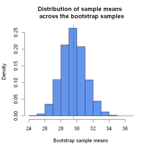
_images/04.e. Population.and.samples_7_0.png

We see a number of features from the graph above;

- The histogram follows an approximately normal distribution (has a symmetric bell-shape)
- It is centred around the sample mean age (from the original sample, \(\hat{\mu} = 29.57\))
- The code below tells us that the standard deviation of this distribution is 1.51.

sqrt(var(r.mean))

1.50868637530863

So we have seen that the bootstrap approximation of the distribution of \(\hat{\mu}^*\) given \(\hat{\mu}\) is a normal distribution centred around \(\hat{\mu}\) with standard deviation of 1.51. The bootstrap principle tells us that the distribution of \(\hat{\mu}\) given \(\mu\) is approximately the same. In other words, approximately:

\[ \hat{\mu} \sim N(\mu, 1.51^2) \]

Remember, that we obtained the true distribution algebraically above and found that

\[ \hat{\mu} \sim N(\mu, 1.52^2) \]

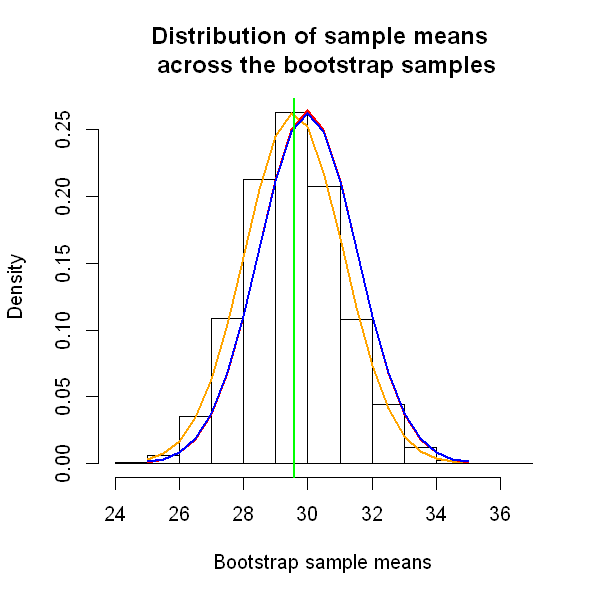
So the resampling (bootstrap) approach has given us a very good approximation to the true sampling distribution. The code below redraws the histogram above, with the approximate (bootstrap) sampling distribution and the algebraically-calculated one.

We see that the bootstrap sampling distribution (shown in red) is simply a shift of the normal distribution which best follows the histogram (shown in orange), and that the bootstrap and true (algebraic, shown in blue) sampling distributions are very similar.

# Histogram of estimates (sample means) in bootstrap samples
options(repr.plot.width=5, repr.plot.height=5)
hist(r.mean, freq=FALSE, main="Distribution of sample means \n across the bootstrap samples", xlab="Bootstrap sample means")

# Add the normal distribution which most closely follows the histogram
lines(seq(25, 35, by=.5), dnorm(seq(25, 35, by=.5), mean(ages), 1.52), col="orange",lwd=2)

# Add the bootstrap approximation to the sampling distribution: normal distribution with mean mu=30 SD=1.51
lines(seq(25, 35, by=.5), dnorm(seq(25, 35, by=.5), 30, 1.51), col="red",lwd=2)

# Add the algebraic sampling distribution: normal distribution with mean mu=30 SD=1.52
lines(seq(25, 35, by=.5), dnorm(seq(25, 35, by=.5), 30, 1.52), col="blue",lwd=2)

# Add a vertical line at original sample mean
abline(v=mean(ages),col="green",lwd=2)

_images/04.e. Population.and.samples_11_0.png

4.4.5 What do we use a sampling distribution for?¶

In practice, we have a single sample of data and a single estimate from that sample of the population parameter of interest. When we present our single estimate of a population quantity, we need to be able to say something about how precise it is. Is it likely to be close to the true value? Can we provide a range of values within which we believe the true value lies?

We can only answer these questions, within the framework of frequentist statistical inference, by thinking about what estimates we might have got had we chosen a different sample. This leads us to the sampling distribution - the distribution of the estimator across samples.

In subsequent sessions we will see how the sampling distribution allows us to

construct confidence intervals for population parameters (intervals within which we believe the true value is likely to lie)
conduct hypothesis tests for population parameters

Statistics for Health Data Science