13.6 Including higher-order terms
As we have already discussed, linear regression assumes that the relationship between the outcome and the independent variables is linear. As we already know, this is not always the case in real data. For example, suppose we are interested in the association between weight and age. On average, the weight of young adults will increase with age. However, at a certain age, the average weight may start to decrease. In this case, the association between weight and age would follow a non-linear (upside-down) \(u\)-shape. It could still be possible to model this relationship within the linear regression framework, by adding a second-order term to the model. This procedure is known as quadratic regression.
13.6.1 The quadratic regression model
The quadratic regression model is a multivariable regression model with two independent variables where the second variable is the square of the first variable. Algebraically:
Despite the fact that one of the variables is the square of the other, this is still a linear regression model because the expectation of the outcome is a linear function of both parameters.
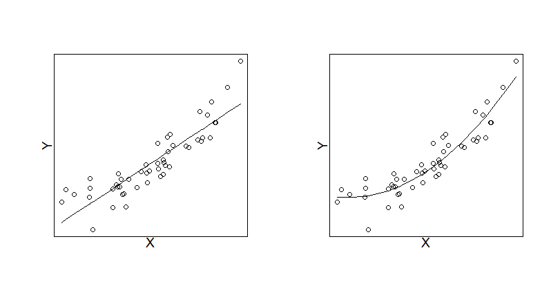
The figure below shows two scatter plots of the data used in Scenario A above. The plot on the left-hand side includes the fitted values of a linear regression model (with no higher-order terms included) and the right-hand side plot includes the fitted values of a quadratic regression model. By comparing the plots, we can see that the quadratic regression model does have a better fit, particularly at the extreme values of \(X\).
Unfortunately, interpreting \(\beta_1\) and \(\beta_2\) is not as straightforward as in most linear models. The reason for this is that it is not possible to change \(X^2\) by 1 unit whilst holding \(X\) constant.
13.6.2 Example
Suppose the outcome, birthweight, is denoted \(Y\) and length of pregnancy (gestational days) is denoted by \(L\). The original linear model we considered was:
We now extend this to allow a quadratic relationship between \(L\) and \(Y\):
# What are the mean gestational days and mothers height in our data?
data<- read.csv('https://www.inferentialthinking.com/data/baby.csv')

# Add quadratic term:
model5<-lm(Birth.Weight~Gestational.Days+I(Gestational.Days**2), data=data)
summary(model5)
Call:
lm(formula = Birth.Weight ~ Gestational.Days + I(Gestational.Days^2),
    data = data)

Residuals:
    Min      1Q  Median      3Q     Max
-49.527 -10.980   0.190   9.973  69.655

Coefficients:
                        Estimate Std. Error t value Pr(>|t|)
(Intercept)           -6.901e+01  5.043e+01  -1.368    0.171
Gestational.Days       8.962e-01  3.678e-01   2.436    0.015 *
I(Gestational.Days^2) -7.890e-04  6.731e-04  -1.172    0.241
---
Signif. codes:  0 '***' 0.001 '**' 0.01 '*' 0.05 '.' 0.1 ' ' 1

Residual standard error: 16.74 on 1171 degrees of freedom
Multiple R-squared:  0.1671,	Adjusted R-squared:  0.1656
F-statistic: 117.4 on 2 and 1171 DF,  p-value: < 2.2e-16
The estimated coefficient for the quadratic term is very small (-0.000789). The p-value, testing the null hypothesis that \(H_0: \beta_2 = 0\) is p=0.241, suggesting no evidence against the null hypothesis. Therefore, we conclude there is no evidence of a quadratic relationship.
13.6.3 More complex models
Quadratic regression models are limited in terms of describing relationships between variables in most medical applications. Quadratic functions either increase to a maximum and the decline, or fall to a minimum and then increase. Further, the behaviour of a quadratic is symmetric about the turning point. Such relationships in medical research are rarely plausible.
There are a number of alternative approaches that can be used to model complex relationships between continuous independent variables and the outcome within a linear regression model. Some are discussed below.
The quadratic regression model belongs to a family of polynomial regression models and is the simplest model in that family. Further power terms can be added to the regression model in order to increase complexity. For example, a cubic regression model is one which includes a cubic term as well as a squared term.
An even more flexible approach is to use a piecewise polynomial model, which allows for a different polynomial function in different ranges of the observed values of \(X\), defined according to specified knots. The flexibility of the model (and therefore its ability to model more complex relationships) can be increased by increasing the degree of polynomial and/or the number of knots. However, highly flexible models may overfit the data and make the model difficult to interpret. In general, it is a good idea to consider an appropriate trade-off between flexibility and interpretability
A related idea is to use splines to flexibly model the relationship. These are a type of piecewise polynomial model, where the adjacent polynomials are constrained to meet at the join points (the knots).