12.3 The simple linear regression model
The equation for the simple linear regression model, relating \(X\) and \(Y\) is:
There are two components of this model: the linear predictor and the error term. The linear predictor represents the variation in \(Y\) that can be predicted using the model: \(\beta_0 + \beta_1 X\). The error term, denoted by \(\epsilon\), represents the variation in \(Y\) that cannot be predicted (by a linear relationship with \(X\)). This variation is sometimes referred to as the random error or noise.
The subsequent two sections take a closer look at the linear predictor and error term, respectively.
12.3.1 The linear predictor
The linear predictor is an additive function of the independent variables. With a single variable, it is simply:
In linear regression, the linear predictor represents the algebraic relationship between the mean of the outcome and the independent variable. When \(X\) takes a particular value, \(X=x\), the value of the linear predictor, \(\beta_0+\beta_1x\), is interpreted as the expected value of \(Y\) when \(X\) takes the value \(x\):
The specification of the linear predictor has two parameters: \(\beta_0\) and \(\beta_1\). These are interpreted as follows:
\(\beta_0\) is the intercept. It is the expected value of \(Y\) when \(X\) takes the value 0.
\(\beta_1\) is the slope (or gradient). It is the expected change in \(Y\) per one unit increase in \(X\).
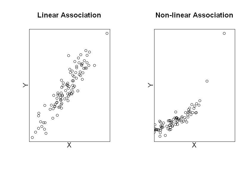
It is worth emphasising that this model assumes that the relationship between \(X\) and \(Y\) is linear. It is important to note that it is possible to have more complex relationships between variables that do not meet this assumption (see examples in the plots below). When this is the case, simple linear regression would not be an appropriate method to use but we might be able to model the relationship well by including non-linear terms. We will pursue these ideas further in the next session.
### Set random number generator
set.seed(24082098)

#Set graphical display to show 2 plots in a row
par(mfrow=c(1,2))
options(repr.plot.height=5)

#Simulate a linear X-Y relationship and plot
x<-rnorm(100,0,1)
ylin<-x+rnorm(100,0,0.5)
plot(x,ylin,xaxt="n", yaxt="n", xlab=" ", ylab=" ", main="Linear Association")
title(ylab="Y", line=0, cex.lab=1.2)
title(xlab="X", line=0, cex.lab=1.2)

#Simulate a non-linear X-Y relationship and plot
ynonlin<-exp(x)+rnorm(100,0,0.5)
plot(x,ynonlin, xlim=c(-0.5,3), yaxt="n", xaxt="n", xlab=" ", ylab=" ", main="Non-linear Association")
title(ylab="Y", line=0, cex.lab=1.2)
title(xlab="X", line=0, cex.lab=1.2)
12.3.2 The error term
The error term, \(\epsilon\) represents the variance in \(Y\) that cannot be predicted by the model. Individual values of the errors can be written as (Y - (\(\beta_0 + \beta_1X\))). These errors cannot be observed, since they involve the unknown population parameters \(\beta_0\) and \(\beta_1\).
We assume that \(\epsilon\) has a normal distribution with mean 0 and variance \(\sigma^2\), where \(\sigma^2\) is termed the residual variance (i.e. the variance of the residuals):
Importantly, note that the errors must be independent of the independent variable \(X\).
12.3.3 Different ways of expressing the simple linear regression model
Suppose we have a sample size of \(n\) and we let \(y_i\) and \(x_i\) \((i=1,...,n)\) denote the observed outcome and value of \(X\) for the \(i^{th}\) observation, respectively. Then, we can write the simple linear regression model as:
Recall that \(iid\) means “identically, independently distributed”. A key assumption of linear regression model is that all of the observations are independent.
This relationship can equivalently be expressed using matrix algebra:
In this formulation, \(\mathbf{X}\) is an \(n \times 2\) matrix, \(Y\) and \(\epsilon\) are vectors of length \(n\) whilst \(\beta\) is a vector of length 2.
12.3.4 Assumptions
It is worth emphasising the four key assumptions that we have made in the simple linear regression model:
Linearity: The relationship between \(X\) and the mean of \(Y\) is linear.
Normality: The errors follow a normal distribution.
Homoscedasticity: The variance of error terms are constant across all values of \(X\).
Independence: All observations are independent of each other.