6.2 Properties of maximum likelihood estimators
Maximum likelihood estimators can be shown to have some very useful properties. In particular, there are some very important asymptotic properties (properties that we observe as the sample size of our data gets very very large).
To explore these properties, have a look at the simulation below. We generate a sample of size 8 from the exponential distribution where \(\lambda=12.22\). The MLE is calculated from this the observed mean of the sample. We repeat this 100 times, and we plot a histogram of the 100 MLEs that we obtain.
Change the sample size, \(n\), to larger numbers and see what you notice about the histogram.
n <- 8  #  make this sample size bigger, and see what happens to the histogram!

# MLEs will be stored in this vector
mle <- rep(0, 100)

for (i in 1:100){
  # Generate a sample of size n from an exponential distribution with lambda=0.0818
  sample <- rexp(n, rate=0.0818)
  # Calculate the MLE (the reciprocal mean of the sample) and store it
  mle[i] <- 1/mean(sample)
}

# Plot a histogram of the 100 MLEs
options(repr.plot.width=5, repr.plot.height=5)
hist(mle, breaks=20,
     xlim=c(0, 0.3),
     main="Histogram of MLE",
     xlab="MLE")
# Add red line to indicate true lambda
abline(v=12.22, col="red")
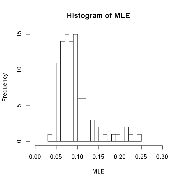
You may notice that, as \(n\) becomes large, the distribution of the MLE becomes more and more concentrated around the true value, and the histrogram appears to look more bell-shaped.
Suppose we denote the parameter of interest as \(\theta\) and its MLE as \(\hat{\theta}\). The tabs below show some important properties of MLEs.
The MLE is asymptotically unbiased, i.e. on average we obtain the correct answer as samples become large.
\(\mathbb{E}(\hat{\theta}) \rightarrow \theta\) as \(n \rightarrow \infty\).
The MLE is consistent, i.e. the MLE converges towards the correct answer as samples become large.
\(\hat{\theta} \rightarrow \theta\) in probability as \(n \rightarrow \infty\).
The MLE is asymptotically normal.
\(\hat{\theta} \sim N(\theta ,Var(\hat{\theta} ))\) as \(n \rightarrow \infty\).
The approximate normal distribution of the MLE means that confidence intervals and hypothesis tests for the parameters can be constructed easily.
The MLE is asymptotically efficient.
\(Var(\hat{\theta})\) is the smallest variance amongst all unbiased estimators as \(n \rightarrow \infty\).
This means that, for example, confidence intervals constructed around the MLE will be the narrowest amongst confidence intervals of estimators that are linear and unbiased.
The MLE is transformation invariant.
If \(\hat{\theta}\) is the MLE for \(\theta\), \(g(\hat{\theta})\) is the MLE of \(g(\theta)\) for any function \(g\).
You might question to what extent these asymptotic properties are useful in practical examples where the sample size is relatively small.
Further, in the cases that we have covered so far, it is fairly straightforward to compute the likelihood function and to find the value that maximizes it, but in many situations, this will be a complex task that requires numerical approaches.
In the subsequent sessions on Bayesian Statistics, we will see a different paradigm for making inference which can address some of these issues.