2.3 The Poisson distribution¶

The Poisson distribution is used to model the number of events occurring in a fixed time interval.

Similarly to our approach with the Binomial distribution, in the following calculations we will assume that we know the true rate at which events occur. In practice, of course, this rate is often the unknown quantity that we are trying to estimate. Later sessions will revisit this example, under the more realistic scenario where this rate is unknown and we are using the sample of data to make inferences about the rate. The calculations in the current session will form important building blocks for those later sessions.

2.3.1 Example of the Poisson distribution¶

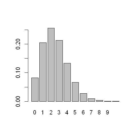
A clinical research is interested in modelling the number of asthma attacks that people with asthma experience in one year. Based on a large sample the researcher has estimated that the average number of attacks in a year is 2.5.

If we let \(X\) be the variable for the number of attacks a randomly selected person with asthma will experience in a year and we are happy to assume that \(X\) follows a Poisson distribution, then we can calculate \(P(X=x)\) for any given value of \(x\).

The code below (in R) does this calculation and plots the probability distribution function of the number of asthma attacks in a year.

# Obtain the probability distribution function (for values x=0,1,...,10)
x <- seq(0,10)
lambda <- 2.5
px <- dpois(x, lambda)

# Create bar chart of PDF
options(repr.plot.width=4, repr.plot.height=4)
barplot(height=px, names=x)

_images/02.d. Probability.Discrete_2_0.png

2.3.2 Deriving the Poisson distribution¶

To give a heuristic derivation of the probability distribution function of the Poisson, we divide the total time \(T\) into a very large number of small intervals (see Figure below). As the number of intervals we divide \(T\) into increases, at most one event will occur in each interval, and so \(X\) will equal the number of intervals in which an event occurs. Since the occurrence of events in each interval are assumed independent of each other, \(X \sim Bin(n,\pi)\), where \(n\) is the number of intervals and \(\pi\) is the probability of an event occurring in any given interval.

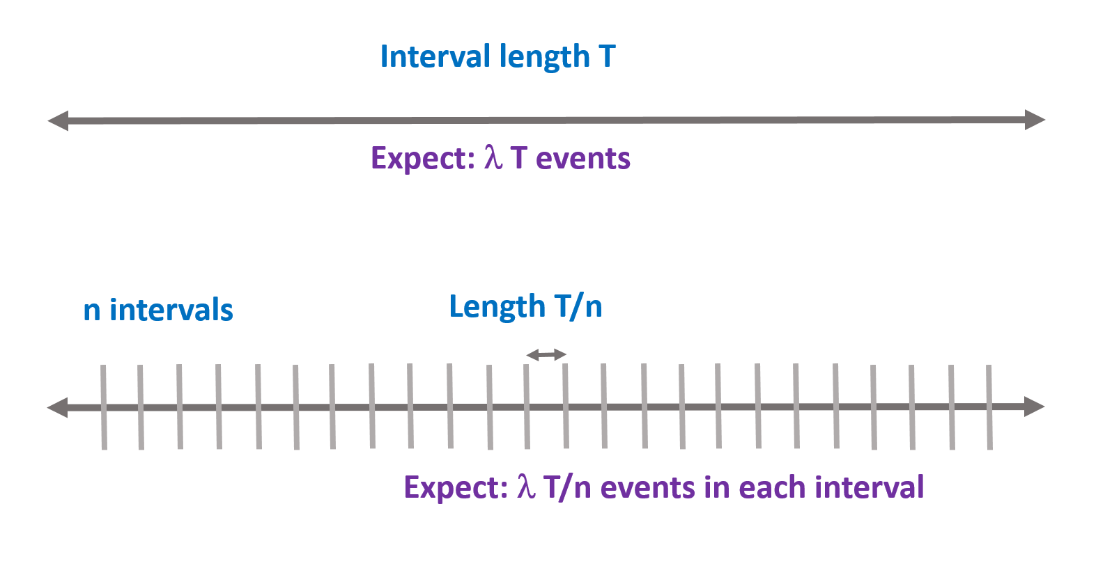
Fig. 1 Derivation of Poisson distribution by dividing time into small intervals¶

With a rate of \(\lambda\) events per unit of time, we expect \(\mu=\lambda T\) events in the whole period, and therefore we expect \(\lambda T / n = \mu/n\) events in each interval. Thus \(\pi=\mu/n\). Therefore, using the probability distribution function for the binomial we have that

\[ P(X=x) = {n \choose x} \pi^{x} (1-\pi)^{n-x} = {n \choose x} \left(\frac{\mu}{n}\right)^{x} \left(1-\frac{\mu}{n}\right)^{n-x} \]

Then we have that

\[ P(X=x) = {n \choose x} \left(\frac{\mu}{n}\right)^{x} \left(1-\frac{\mu}{n}\right)^{n-x} \]

\[ = \frac{n!}{x! (n-x)!} \left(\frac{\mu}{n}\right)^{x} \left(1-\frac{\mu}{n}\right)^{n-x} \]

\[ = \frac{n!}{n^{x} (n-x)!} \frac{\mu^{x}}{x!} \left(1-\frac{\mu}{n}\right)^{n-x} \]

Now to simplify the first term, we note that:

\[ \frac{n!}{n^{x} (n-x)!} = \frac{n(n-1)...(n-x+1)}{n^{x}} \rightarrow 1 \mbox{ as } n \rightarrow \infty, \]

and to simplify the third term, we note that:

\[ \left(1-\frac{\mu}{n}\right)^{n-x} \rightarrow \left(1-\frac{\mu}{n}\right)^{n} \rightarrow e^{-\mu} \]

Replacing the first and third terms by these limits gives

\[ P(X=x) \rightarrow \frac{\mu^{x}}{x!} e^{-\mu} \mbox{ as } n \rightarrow \infty. \]

2.3.3 General form of the Poisson distribution¶

We can now define a Poisson distribution for the number of events occurring in a fixed interval \(T\) at a constant rate \(\lambda\) with parameter \(\mu=\lambda T\), which we write as

\[ X \sim \mbox{Poisson}(\mu=\lambda T) \]

as the distribution which has probability distribution function

\[ P(X=x) = \frac{\mu^{x}}{x!} e^{-\mu}, \ \mbox{ for } x=0,1,2,... \]

Expectation and variance

The derivation of the expectation and variance of a Poisson random variable \(X\) with parameter \(\mu\) will be set as a practical question.

2.3.4 Applications of the Poisson distribution¶

Assumptions

The Poisson distribution is used to model the number of events occurring in a fixed time interval \(T\) when:

events occur randomly in time,
they occur at a constant rate \(\lambda\) per unit time,
they occur independently of each other.

Applications

A random variable \(X\) which follows a Poisson distribution can take any non-negative integer value. Examples where the Poisson distribution might be appropriate include:

Emissions from a radioactive source,
The number of deaths in a large cohort of people over a year,
The number of accidental deaths occurring in a city over a year.

2.3.5 Approximating the binomial by a Poisson¶

When \(n\) is large relative to \(\pi\), the binomial distribution can be approximated by a Poisson with a mean \(n\pi\). That this approximation is reasonable follows directly from our earlier heuristic derivation of how a Poisson distribution arises as an approximation to a binomial distribution when the number of trials tends to infinity.

There are many such approximations. Nowadays, we may not need to use them because we have enormous computing power at our disposal. In earlier times, in contrast, calculations could take a long time so any simplification that could be reasonably applied could provide meaningful extra calculation speed.

Statistics for Health Data Science