6.1 Likelihood with independent observations
Suppose that the observed data consiste of a sample of \(n\) observations. If these observations are independent, then the joint likelihood function from these \(n\) observations has a very convenient form; it is the product of the likelihood from each observation.
Suppose that the random variables \(X_1,..., X_n\) are i.i.d., and that our observed data are \(\mathbf{x} = \left\{ x_1, x_2, ..., x_n \right\}\). Then the likelihood function is given by:
Recall that we often prefer to work with the log-likelihood function, as it simplifies the algebra when it comes to finding the MLE. The log-likelihood function for \(n\) independent observations is given by:
Finding the MLE involves the same three steps as we saw in the previous session, but the log-likelihood function is now a joint function for the \(n\) observations:
Method for finding MLEs:
Obtain the derivative of the log-likelihood: \(\frac{d l(\theta \mid \mathbf{x})}{d \theta}\)
Set \(\frac{d l(\theta \mid \mathbf{x})}{d \theta}=0\) and solve for \(\theta\)
Verify that it is a maximum by showing that the second derivative \(\frac{d ^2 l(\theta \mid \mathbf{x})}{d \theta ^2 }\) is negative when the MLE is substituted for \(\theta\).
6.1.1 Example: Exponential distribution
Recall the example from the previous session, investigating the time that patients wait until their GP appointment in a particular practice. The receptionist records the time that elapses between when a patient walks through the door, and when they are called through for their appointment for a random sample of 8 people. These times (in minutes) are: 8.75, 10.20, 15.29, 7.89, 7.04, 12.04, 19.04, 17.50.
As a reminder, we can model the waiting time until a specific event using the exponential distribution with parameter \(\lambda\), which has a probability density function given by:
Recall that the mean of this distribution is equal to one over the rate parameter \(\lambda\), i.e. \(E(X) = \frac{1}{\lambda}\).
We have that the log-likelihood is:
We can make a plot of this log-likelihood, using the data from our example with eight observations.
options(repr.plot.width=4, repr.plot.height=4)

#six independent observations for waiting times
obs <- c(8.75, 10.20, 15.29, 7.89, 7.04, 12.04, 19.04, 17.50)
n <- length(obs)

#possible values for the parameter lambda
lambda <- seq(0, 2, 0.01)

#plot the log-likelihood
plot(lambda, n*log(lambda) - lambda*sum(obs), type="l",lwd=2,
     xlab= expression(lambda), ylim=c(-100,0),
     ylab="Log-likelihood")
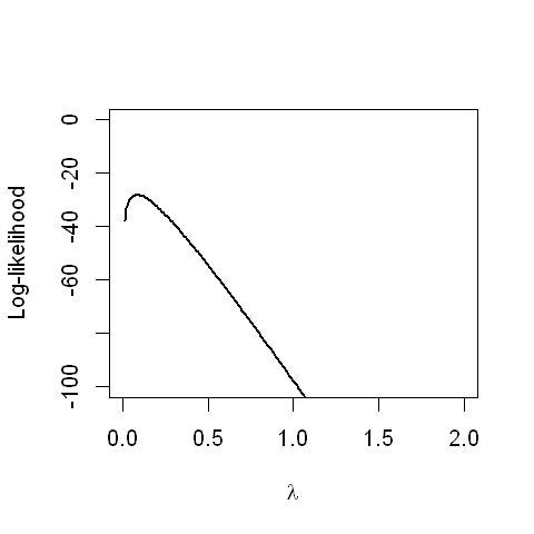
Graphically, we observe that the maximum is between 0 and 0.25. We will use the three steps, as before, to derive the MLE algebraically:
Step1: Taking the derivative of the log-likelihood with respect to \(\lambda\):
Step2: Set the derivative equal to zero and solve for \(\lambda\):
The MLE is \(\hat{\lambda}= \frac{1}{\bar{x}}\). And to check that this provides a maximum, we go on to the next step:
Step3: Find the second derivative:
When \({\lambda}=\frac{1}{\bar{x}}\), we have:
which is negative. This verifies that we found the maximum likelihood estimate.
Going back to our example of eight patients waiting for their GP appointment, the maximum likelihood estimate \(\lambda\) is given by one over the average of the eight waiting times:
1/mean(obs)
We have that \(\hat{\lambda}=0.0818\) minutes.
6.1.2 Example: Normal distribution
We will now consider the normal distribution. Remember that the normal distribution has two parameters, \(\mu\) and \(\sigma^2\). We will first obtain the MLE for \(\mu\) (treating \(\sigma^2\) as a constant), and in the practical, we will obtain the MLE for \(\sigma^2\) (treating \(\mu\) as a constant).
Recall that normal distribution has probability density function given by*:
(* note that the notation here is slightly different to section 3. Here we are more prescriptive; on the left hand side the notation says that the random variable \(X\) is sampled from parameters \(\mu\) and \(\sigma^2\), where the distribution is defined on the right hand side. Both versions of notation are acceptible. Another notation style is to use a semi-colon instead, ie. \(f_X( x ; \mu, \sigma^2)\)).
We have that the log-likelihood given an i.i.d. sample of size \(n\) is:
We will first find the MLE for the parameter \(\mu\).
Step1: Take the derivative of the log-likelihood with respect to \(\mu\). Note that this requires use of the chain rule:
Step2: Setting the derivative equal to zero and solving for \(\mu\):
Since \(\sigma^2 > 0\), we have that:
We have that the MLE for \(\mu\) is the sample mean, \(\bar{x}\).
Step3: Find the second derivative:
since both \(n>0\) and \(\sigma^2 >0\), we have that the second derivative is negative, verifying that we have found the maximum.
In the practical, we will find the MLE for \(\sigma^2\).