7.3 Interpretation of confidence intervals
For our emotional distress sub-sample, our estimated mean age is \(\hat{\mu}= 29.75\), with a 95% confidence interval of \((26.6, 32.5)\). Having calculated this confidence interval for our unknown population age, \(\mu\), how do we interpret it?
7.3.1 Operational definition
For the 95% confidence interval calculated above \((26.6, 32.5)\), it is tempting to say that the probability that the population mean age, \(\mu\), is between 26.6 and 32.5 is 95%. However, this is incorrect, because this implies that \(\mu\) has a probability distribution, rather than being a fixed unknown number. Either the true value of \(\mu\) lies within the interval 26.6 to 32.5, or it does not.
Strictly, the interpretation of a confidence interval has to be with respect to the process of repeated sampling: if we repeated the study an infinite number of times, 95% of the 95% confidence intervals calculated would include the true population mean \(\mu\).
This operational definition is long-winded and can be confusing. In practice, we often use looser interpretations to aid communication of results, as described below.
7.3.2 Looser interpretation (practical)
In practice, we often loosely interpret a 95% confidence interval by saying
that we are 95% confident that the true population mean lies within the 95% confidence interval calculated.
that our data are consistent with values of the population mean within the 95% confidence interval calculated.
It is important, however, to bear the strict operational definition of the confidence interval in mind when we use these types of interpretations.
7.3.3 Confidence intervals under repeated sampling
In order to see how confidence intervals behave under repeated sampling, we will now randomly draw 100 different samples of 10 people. Within each sample, we calculate the sample mean and the 95% confidence interval (assuming the population value \(\sigma\) is known). The graph below shows the 95% confidence intervals from the 100 samples. [Click to view the code that generates the graph].
# Population parameters
mu <- 30
sd <- 4.8
n_in_study <- 10

# Take 100 samples of 10 people, measure ages in each set of 10 people
different_studies <- 100
set.seed(1042)
study_measurements_age <- list()
for (i in 1:different_studies) {
  study_measurements_age[[i]] <-  rnorm(n_in_study, mu, sd)
}

# Calculate sample means and 95% confidence intervals
sample.means   <- sapply(study_measurements_age, mean)
sample.cl   <- sapply(study_measurements_age, function (x) mean(x) - 1.96*1.52)
sample.cu   <- sapply(study_measurements_age, function (x) mean(x) + 1.96*1.52)

# Extract means and CIs for samples which miss the true value
out <- ((sample.cl>30) + (sample.cu<30))
out.means <- sample.means[out==1]
out.cl <- sample.cl[out==1]
out.cu <- sample.cu[out==1]
out.samples <- seq(1,100,1)[out==1]

# Graph all the sample means and CIs
options(repr.plot.width=5, repr.plot.height=6)
plot(sample.means, seq(1,100,1), main="95% confidence intervals for the mean age", xlab="Mean age (years)", ylab="Sample", xlim=c(22, 38), ylim=c(0, 100), yaxt="none")
abline(v=30)
for (i in 1:100) {
  eval(lines(c(sample.cl[i], sample.cu[i]), c(i, i)))
}

# Highlight the CIs that miss the true value in red
points(out.means, out.samples, col="red")
for (i in 1:length(out.samples)) {
  eval(lines(c(out.cl[i], out.cu[i]), c(out.samples[i],out.samples[i]), col="red"))
}
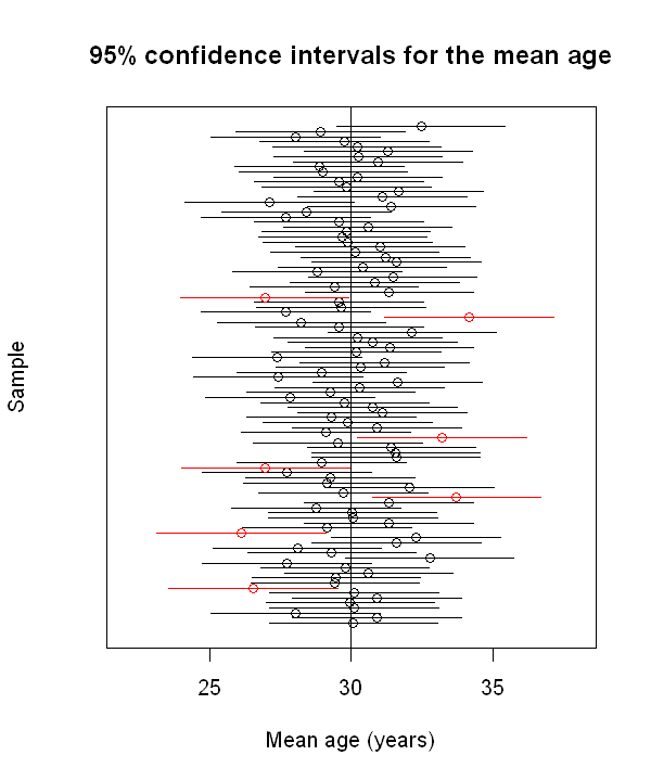
In the figure above, what do you notice? Approximately what proportion of intervals include the true value of \(\mu\)? Have a think about this and then click to see some comments about the graph.
We see that:
the point estimates tend to cluster around the true value of \(\mu\), and fall symmetrically either side
93 out of the 100 confidence intervals include the true value
3 out of 100 of the intervals to lie entirely above the true value
4 out of 100 of the intervals to lie entirely below the true value
If we were to do simulate a much larger number of confidence intervals, we would see that:
95% of the confidence intervals would include the true value
2.5% of the intervals would lie entirely above the true value
2.5% of the intervals would lie entirely below the true value