9.1 Introduction to Bayesian Inference
9.1.1 Probability
In Session 2, we learned about probability in the frequentist sense: the proportion of times an event occurs in the long-run. Let’s have a look at the following two scenarios:
A research group wishes to know the probability that a baby who is born in a particular hospital ward has cystic fibrosis. They look at the records on screening tests done at birth to investigate.
A 34 year old woman attends her GP practice, worried that she has cancer because she has had feelings of “fullness” and “bloating” as well as mild nausea for the last 2 weeks. The patient mentions ovarian, bowel and pancreatic cancer as concerns having read about her symptoms on the internet. The rest of the history as well as physical examination are unremarkable. If the GP’s assessment of the risk were above a certain level, the GP might refer the patient for tests (collect more data). In this case, the GP concludes that the current information about the patient suggests there is a very low risk that the patient has cancer.
What is the quantity that we trying to estimate in each scenario?
What is the frequentist definition of probability in each of these settings? Does it make sense?
A key problem with the frequentist paradigm is that the “long-run” frequency definition is not always relevant, or even appropriate, as we see in the second example above. Further, notice that the GP uses information from different sources to draw his/her conclusion about the probability that the patient has cancer. This synthesis of information can be incorporated into a Bayesian framework. A frequentist, in contrast, would tackle this problem by thinking about:
a) the probability of the patient having these symptoms, given that she has cancer;
b) the probability of the patient having these symptoms, given that she does not have cancer;
and comparing the two probabilities. Note that this does not take into account the extra information about the context.
9.1.2 Bayesian Inference
The underlying concept for Bayesian inference essentially works as follows. We have some population parameter \(\theta\) which we wish to make inference on, and the likelihood \(p(y|\theta)\) which tells us how likely different values of \(y\) are, conditional on different parameter values \(\theta\). In the frequentist approach, \(\theta\) is considered to be a fixed, but unknown, constant. Inference is then based on the likelihood \(p(\mathbf{y}|\theta)\), where \(\mathbf{y} = \left\{y_1, . . . ,y_n\right\}\) is a sample of observations from the population. The frequentist approach looks at the distribution of the data given \(\theta\) to estimate \(\theta\) by using, for example, the maximum likelihood approach which we covered in Session 6.
In the Bayesian paradigm, we no longer assume that the parameters have a fixed true value, but consider \(\theta\) to be a random quantity with an unknown distribution, which we wish to estimate. This distribution is denoted by \(p(\theta|y)\), and so we look at the distribution of the parameter, having seen data \(y\). To achieve this, we will have to specify a prior probability distribution, denoted \(p(\theta)\), which represents our initial beliefs about the distribution of \(\theta\) prior to observing any data. In some situations, when we are trying to estimate a parameter \(\theta\) we have some knowledge, about the possible value of \(\theta\) before we take into account the data that we observe.
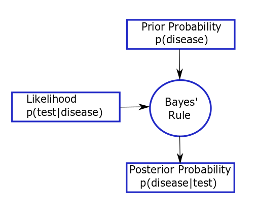
For example, consider the way a physician makes diagnostic decisions. A patient presents with a set of symptoms, concerned that they might have a certain disease. The physician assesses the probability that this patient has this disease, based on symptoms, family history, alternative explanations of symptoms and prevalence of the disease (their prior view that the patient has the disease). The physician might send the patient for a diagnostic test (collects some data) if her prior assessment of risk is above some threshold. Then the physician re-assesses the chance that the patient has this disease, taking account of the results and reliability of the diagnostic test (updates their prior in light of the data to get a posterior view on whether the patient has the disease). Depending on their certainty, the physician may then send the patient for further diagnostic tests. This thought process can be represented by the figure below and is analogous to Bayesian thinking.
In this example, the physician is assessing the probability that the patient has the disease. It is the physician’s prior probability based on their own training, knowledge and experience; a colleague may have a different prior probability. Here, prior probability is being defined subjectively. The size of the probability represents the physician’s degree of belief about the occurrence of an event, i.e. their own personal assessment of how likely an event is, based on the evidence available to them before the test results are given. This definition corresponds more closely to the everyday, intuitive usage of probability than a frequentist interpretation (where the probability of a particular event occurring can be interpreted as the proportion of times the event would/does occur in a large number of similar trials or situations). The prior probability of the event might come from direct data, known prevalance of disease in a population, or data from related populations. If such prior information does not exist, then it can be formally elicited from experts, but we would want to acknowledge the uncertainty in the experts’ knowledge.