12.5 Example: continuous independent variable
We now return to our first example, where we are interested in investigating the association between birthweight and length of pregnancy. We will fit a linear model to explore this association.
12.5.1 The model
The outcome is birthweight, which is measured in ounces (oz). The independent variable is length of pregnancy, \(L\) (i.e. number of gestational days).The following model defines our assumed relationship between the length of pregnancy (\(L\)) and a baby’s birthweight (\(Y\)):
We will use the lm() to perform simple linear regressions in R. Click here for details of how this command works.
The following code can be used to perform this linear regression in R:
# Model 1: Investigating the relationship between birthweight and length of pregancy
data<- read.csv('https://www.inferentialthinking.com/data/baby.csv')
model1<-lm(Birth.Weight~Gestational.Days, data=data)
summary(model1)
Call:
lm(formula = Birth.Weight ~ Gestational.Days, data = data)

Residuals:
    Min      1Q  Median      3Q     Max
-49.348 -11.065   0.218  10.101  57.704

Coefficients:
                  Estimate Std. Error t value Pr(>|t|)
(Intercept)      -10.75414    8.53693   -1.26    0.208
Gestational.Days   0.46656    0.03054   15.28   <2e-16 ***
---
Signif. codes:  0 '***' 0.001 '**' 0.01 '*' 0.05 '.' 0.1 ' ' 1

Residual standard error: 16.74 on 1172 degrees of freedom
Multiple R-squared:  0.1661,	Adjusted R-squared:  0.1654
F-statistic: 233.4 on 1 and 1172 DF,  p-value: < 2.2e-16
There is a lot of information contained in this output. For the moment, we will focus on the estimates of the intercept and slope. These can be found under the column heading Estimate.
The estimated intercept, \(\hat{\beta}_0\) is equal to -10.75. This is interpreted as: the estimated mean birthweight of a child born after 0 gestational days is -10.75oz. Since there are no observations with 0 gestational days in the study, this is an extrapolation based on the observed data and an assumption of linearity. Estimates based on extrapolation should be interpreted with caution and in this case, the results make little sense because a negative birthweight is estimated. Moreover, no child is born after 0 gestational days and so this intercept is of little interest. Later on, we will discuss a technique called centering which is often used to make the intercept term more interpretable.
The estimated slope, \(\hat{\beta}_1\) is equal to 0.47. This is interpreted as: the mean birthweight of a baby is estimated to increase by 0.47oz for each daily increase in the gestational period.
The estimated residual standard error, \(\hat{\sigma}\) is equal to 16.74 (the residual variance is equal to \(16.74^2\)). This means that the observed outcomes are scattered around the fitted regression line with a standard deviation of 16.74oz.
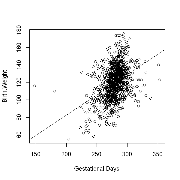
It is always useful to look at the data. The code below graphs the data and superimposes the fitted regression line.
options(repr.plot.width=5, repr.plot.height=5)
with(data, plot(Gestational.Days, Birth.Weight))
abline(model1)