4.1 Sampling from a population
Much of statistical inference is concerned with making statements about properties of populations, based on properties of samples from the populations. A helpful mental picture of the population and the sample to have in mind is as follows. Imagine that the population is a very large number of “objects” contained in a large urn, from which we can randomly sample a relatively small number of the “objects” at a time to provide our sample.
The objects in our population are often called sampling units. For many health research questions these sampling units are individual patients. If we were collecting information about different hospitals in order to make comparison between different providers, then the sampling unit might be hospitals.
Making statements about a population using information contained in a sample of data relies critically on the process of how the sample was drawn from the population (i.e. the sampling process). A common example of a sample process is random sampling. Under random sampling, each object in the population has the same chance of appearing in the selected sample. Inference procedures tend to be most straightforward in this setting.
In many cases, sampling is not random. For example, many populations have intrinsic structure that might facilitate sampling. If our population is people in rural Gambia, for example, then the easiest way to sample individual people might be to choose 5 villages and then go and survey the people in those villages. While it is not necessarily difficult to modify the process of statistical inference for such situations, statistically invalid conclusions can be reached if such modifications are not undertaken.
4.1.1 Parameters and estimators
In statistical inference, the aim is to make statements about certain features of the population, using the information contained in the sample data. Typically, we quantify the features of interest in terms of unknown population quantities (some examples might be a population mean, standard deviation, proportion, or risk ratio) and attempt to estimate these population quantities. We call these unknown population quantities population parameters. Parameters are typically denoted using Greek letters. Often, certain letters tend to be used for certain types of quantities. For instance, \(\mu\) will often denote a population mean and \(\pi\) will often denote a population proportion. When we are talking about a general “parameter of interest”, we often use the letter \(\theta\).
A statistic, is any quantity that can be calculated from the known measurements on the sample data. It can be any function or combination of random variables that does not depend on unknown parameters for its calculation. As for population parameters, certain letters tend to be used for certain sample statistics. For instance, \(\bar{x}\) (“x bar”) will often denote a sample mean and \(p\) a sample proportion.
We often want to estimate a population parameter from the sample. We do this by using sample statistics to estimate population parameters. For example, the obvious statistic to use to estimate a population mean is the sample mean. When a sample statistic is used for the purpose of estimating a population parameter it is known as an estimator. So an estimator is a statistic that is designed to be a “guess” at a particular parameter of a population. When we use a sample statistic to esitmate a population parameter we use a “hat” to denote the estimator, e.g. \(\hat{\mu}\) is an estimator for the population quantity \(\mu\) and \(\hat{\theta}\) is an estimator for the population quantity \(\theta\).
Once we have drawn our sample of data and calculated the value of the estimator in that sample, we refer to this as the estimate. In other words, the term estimate is used for the value obtained by substituting sample data values into the formula for the estimator.
The basic structure of frequentist inference can be represented diagrammatically as follows:
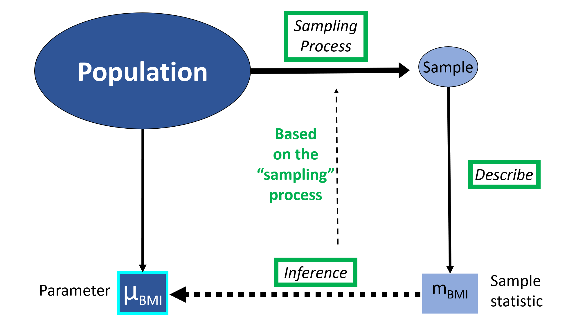
Fig. 2 Statistical inference
4.1.2 Example
To explore these issues further, we will consider a study question investigated by a recent MSc student at LSHTM as part of their summer project. The student explored the question of whether people who engage with victims of violence themselves suffer from emotional distress. This question was assessed using a sample of 53 violence researchers in Uganda. Subsequently, these violence researchers took part in a randomised trial, but we will focus on the initial description of the sample. The full article can be found here https://www.ncbi.nlm.nih.gov/pmc/articles/PMC5455179/
For the purposes of illustration, in this session we will take a smaller sample of 10 violence researchers. Among our 10 sampled violence researchers, the sample mean age and the sample proportion suffering from emotional distress are
Sample mean age \(\bar{x}= 29.75\); sample standard deviation of age \(SD = 4.49\)
Proportion suffering from emotional distress \(p = 26\%\) (14 out of 53)
Let \(X_1, ..., X_{10}\) be random variables representing the ages of 53 sampled researchers. In other words, \(X_1, ..., X_{10}\) represent the random process by which the eventual 10 values of age are obtained. We call the realisation of these random variables (i.e. the observed data) \(x_1, ..., x_{10}\).
We will initially focus on the population mean age (\(\mu\)) and its estimator. The obvious estimator for the population mean age is the sample mean age. In terms of the general random variables \(X_1, ..., X_{10}\), we can write this estimator as,
This is a random variable representing the mean of the random variables \(X_1\),…,\(X_{10}\). The sample statistic estimate is,
The estimate is the sample mean age, which is the realisation of \(\bar{X}\) in the observed data. Since we are now viewing this as an estimate of \(\mu\), we can also write \(\hat{\mu} = \bar{x}\).
Discussion question
- From above, our “best guess” at (our estimate of) the population mean age is 29.75.
- Is this estimate a “good” estimate of the population mean? Do we think it is close to being correct?
- If we sampled a different 10 researchers would we be likely to see a similar sample mean age? Or could we see a very different sample mean? Is it possible that, just by chance, this is a particularly old (or young) group of researchers?