5.1 Maximum likelihood estimation
Suppose we are interested in the probability that a single patient will experience a particular side effect from a particular drug. We decide to run a small clinical study including 8 patients. The observed data consist of the number, of those 8 patients, who experience a side effect. Suppose that we conduct the study and observe that 2 patients experience a side effect. We wish to use these observed data to make statements - inferences - about the unknown probability of experiencing a side effect from that drug.
Statistical model: We begin by defining a model for the data. Here, we define \(X\) as the random variable representing the total number of the 8 patients who experience a side effect. Our model is that
which - we remember from the probability sessions - involves the assumptions that each Bernoulli event (whether or not each individual patient experiences a side effect) is independent and has the same probability of occurring.
This model involves the unknown parameter \(\pi\).
Data: We have observed a realisation from this model, \(X=2\). These are often called our observed data.
Under our proposed statistical model, the probability that 2 out of 8 patients experience a side effect is:
Since \(\pi\) is unknown, it is natural to consider how the probability of observing these data varies with different values of \(\pi\):
\(\pi\) |
P(\(X\)=\(2\)) |
|---|---|
0 |
0 |
0.25 |
0.311 |
0.5 |
0.109 |
0.75 |
0.004 |
1 |
0 |
Suppose that, in truth, the unknown probability of a patient experiencing a side effect from this drug was 0.75. The probability of then observing 2 from 8 patients experiencing a side effect is 0.004. This is a very low probability, so this would be an unusual or perhaps unexpected event, although not strictly impossible.
Suppose that, conversely, the unknown probability of a patient experiencing a side effect from this drug was actually 0.25. Then the probability of observing 2 from 8 patients experiencing a side effect would be 0.31 (\(31\%\)). If this were the case, there would be nothing unusual or unexpected about our observed data.
We do not know which value of \(\pi\) is the true value. But a sensible strategy to obtain a ‘best guess’, or estimate, of \(\pi\), might be to pick the value which maximises the probability of observing the data that we observed. We will see below that this probability is in fact the likelihood, leading to the concept of maximising the likelihood or maximum likelihood. This is a term that you will encounter frequently in statistics.
Following these ideas, we can extend the table above by considering a finer range of possible values for \(\pi\) between 0 and 1, and plot the probability of observing \(X=2\), assuming that that value of \(\pi\) were true. This gives the graph below.
# Define a range of values for pi
pi = seq(0,1,by = 0.05)

# Calculate the likelihood for each value, given n=8 and x=2
L_pi <- choose(8,2)*pi^2*(1-pi)^(8-2)

# Plot the output
options(repr.plot.width=5, repr.plot.height=5)
plot(x = pi, y = L_pi)

# Add a line to indicate the value which yields the highest likelihood
abline(v = pi[which.max(L_pi)], col = "red")
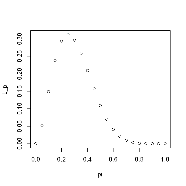
We see that \(\pi=0.25\) is the value that leads to the highest probability of observing the data that we did indeed observe (i.e \(X=2\)) so we choose this value as our best guess for \(\pi\). We will see that this value is called the maximum likelihood estimator. We write \(\hat{\pi} = 0.25\), where we have added a hat to indicate that this is being viewed as an estimate of an unknown parameter.
The likelihood when \(\pi = 0\) is exactly zero, as is the likelihood when \(\pi = 1\). This makes sense because these two probabilities would make the observed data impossible - they imply that patients would either never or always experience side effects. Informally, we could say that these values are inconsistent with the data.
Note that, our estimate of the probability of a patient experiencing a side effect is intuitively a sensible one: it is the sample proportion, \(\frac{2}{8}\).
We will see later on that estimators obtained in this way (by maximising a likelihood) have very nice statistical properties.