3.3 Uses of the standard Normal distribution
Suppose we wanted to answer the following question:
What is the probability of having a ‘healthy’ weight?
A healthy weight is often is often measured using the Body Mass Index (BMI - although see here and here for a discussion on why this may be too simplistic a measure). An individual’s BMI can be calculated using their height and weight, using the formula BMI \(= \frac{mass(kg)}{height(m)^2}\). Then people can be classified as:
Classification |
BMI |
|---|---|
Underweight |
<18.5 |
Normal |
18.5-24.9 |
Overweight |
25-29.9 |
Obese |
30-39.9 |
Extremely obese |
>40 |
To address our question, we will use data taken from a study undertaken among a group of 76 cleaners, that investigated whether telling the cleaners they had an active lifestyle influenced their BMI. We will assume that values of BMI approximately follow a normal distribution. We do not know the true values of \(\mu\) and \(\sigma\) so we will replace these with the sample mean and standard deviation. This gives us values of \(\mu=\)26.5 and \(\sigma^2=\) 18.1, as demonstrated in the snippet of code below.
# BMI dataset
dat <- read.csv("Practicals/Datasets/BMI/MindsetMatters.csv")
head(dat)
#remove observations with no BMI data
dat <- dat[!is.na(dat$BMI),]
#estimate mu and sigma
mu <- mean(dat$BMI)
print(paste0("value of mu is ",round(mu,2)))
sig <- sd(dat$BMI)
print(paste0("value of sigma is ",round(sig,2)))
| Cond | Age | Wt | Wt2 | BMI | BMI2 | Fat | Fat2 | WHR | WHR2 | Syst | Syst2 | Diast | Diast2 |
|---|---|---|---|---|---|---|---|---|---|---|---|---|---|
| 0 | 43 | 137 | 137.4 | 25.1 | 25.1 | 31.9 | 32.8 | 0.79 | 0.79 | 124 | 118 | 70 | 73 |
| 0 | 42 | 150 | 147.0 | 29.3 | 28.7 | 35.5 | NA | 0.81 | 0.81 | 119 | 112 | 80 | 68 |
| 0 | 41 | 124 | 124.8 | 26.9 | 27.0 | 35.1 | NA | 0.84 | 0.84 | 108 | 107 | 59 | 65 |
| 0 | 40 | 173 | 171.4 | 32.8 | 32.4 | 41.9 | 42.4 | 1.00 | 1.00 | 116 | 126 | 71 | 79 |
| 0 | 33 | 163 | 160.2 | 37.9 | 37.2 | 41.7 | NA | 0.86 | 0.84 | 113 | 114 | 73 | 78 |
| 0 | 24 | 90 | 91.8 | 16.5 | 16.8 | NA | NA | 0.73 | 0.73 | NA | NA | 78 | 76 |
[1] "value of mu is 26.46"
[1] "value of sigma is 4.25"
So what is the probability a randomly selected person in this sample has a normal BMI?
Approach 1: Manual calculation
One option is to make use of pre-calculated probabilities of the standard normal distribution. If we write \(X\) to represent the value of a person’s BMI, then we are assuming that
To make use of the pre-calculated probabilities for the standard normal distribution, we must first transform our normally distributed variable to have a standard normal distribution. We know that the transformed variable \(Z\) (the Z score) has a standard normal distribution, where
Given values for \(\mu\) and \(\sigma\) we can go from the X scale to the Z scale and vice versa. The important point about describing a distribution on the Z scale is that this opens the ability to calculate specific probabilities. So back to answering the question…
From the table above we can see that a normal weight is classified as a BMI between 18.5 and 24.9, and we want to know what the probability is that a randomly selected person falls between these limits. We write this as;
On the Z-scale, this is equivalent to saying that:
Tables exist containing a range of pre-calculated probabilities that a variable following a standard normal distribution takes a value of less than \(k\), for a range of possible values of \(k\). These are often called z-tables (found online or at the back of most stats books). From these tables, we can look up the corresponding probability for each z-score, giving:
Approach 2: Using R to do the same calculation
Using this approach, R is ultimately using the same pre-calculated probability tables. However, it is considerably quicker and easier to ask R to look up the values rather than finding them in tables.
# a) if we were to use Z tables within R (to illustrate the point)

z_min <- (18.5-mu)/sig
z_max <- (24.9-mu)/sig

# note when using pnorm we don't need to specify mu and sigma as the
# function assumes mu=0 and sigma=1 unless specified.
print(paste0("z_max is ",round(z_max,2)," and z_min is ",round(z_min,2)))
print(paste0("Probability of having a healthy BMI is (z-score) ",round(pnorm(z_max)-pnorm(z_min),3)))
[1] "z_max is -0.37 and z_min is -1.87"
[1] "Probability of having a healthy BMI is (z-score) 0.326"
Approach 3: Using R to do the calculation on the untransformed scale
# b) if we were to directly estimate

print(paste0("Probability of having a healthy BMI is (direct) ",round(pnorm(24.9,mu,sig)-pnorm(18.5,mu,sig),3)))
[1] "Probability of having a healthy BMI is (direct) 0.326"
Calculating directly gives the same result as using a z-score in R, and this returns the same information as using z-tables.
In answer to our question, we estimate that the probability of having a ‘healthy’ weight is 32.6%. We can compare this to the observed proportion of our sample of data with a ‘healthy’ BMI.
# c) provide a sanity check against the data
options(repr.plot.width=4, repr.plot.height=3)
library(ggplot2)

ggplot(dat,aes(x=BMI)) + geom_histogram(bins = 30,fill="steelblue",col="grey80") +
    geom_vline(xintercept = c(18.5,24.9))
#hist(dat$BMI,col="steelblue")
#abline(v=c(18.5,24.9),lty=2)
print(paste0("Within the data a healthy BMI is seen ",
             round(100*((sum(dat$BMI<24.9)-sum(dat$BMI<18.5))/length(dat$BMI)),1),"%"))
[1] "Within the data a healthy BMI is seen 35.1%"
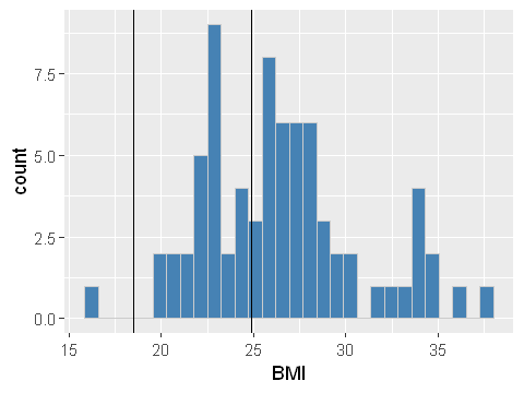
So we can see that the sample estimate (35.1%) is roughly similar to the population estimate of 32.6%.