7.1 Confidence intervals
To explore the concept of confidence intervals, we will return to the example of emotional distress among violence researchers.
We will again consider the smaller subsample of 10 researchers and focus on estimating the population mean age, \(\mu\). Among our 10 sampled violence researchers, the sample mean age and the sample proportion suffering from emotional distress are:
Sample mean age \(\bar{x}= 29.57\); sample standard deviation of age \(SD = 4.95\)
Statistical model: As before, we will let \(X_1, ...,X_{10}\) be random variables representing the ages of 10 sampled researchers . For simplicity, we will assume that we know the true value of the population standard deviation, \(\sigma = 4.8\). We assume the following model
Data: The realised values of the random variables are \(x_1, ..., x_{10}\) (i.e. the observed ages).
Estimator and estimate: The best estimator of the population mean age is the sample mean age.
From our sample of data, the estimate is \(\hat{\mu} = 29.57\). But how good an estimate is this? In order to answer that question, we will construct a 95% confidence interval around the estimate.
Sampling distribution of the estimator: Recall that the sampling distribution of the sample mean is the distribution we would see if we repeatedly sampled 10 researchers a very large number of times, each time calculating the sample mean age, and drew a histogram of the sample means. We obtained the sampling distribution algebraically:
Recall that when we are talking about the sampling distribution (i.e. the distribution of an estimator), we call the standard deviation the standard error. So the sample mean age follows a normal distribution, under repeated sampling, centred around the population mean \(\mu\) with standard error given by \(SE(\hat{\mu}) = 1.52\).
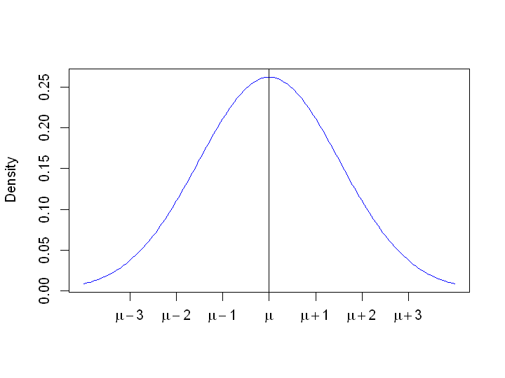
We do not quite have sufficient information to plot the sampling distribution, because we still do not know where the central value \(\mu\) is. However, otherwise we can draw the exact shape. The graph below draws the sampling distribution around an unknown population mean \(\mu\).
[The code used to generate the graph is suppressed, since it is not our focus here, but if you wish to see it you can click the button to the right.]
# Labels for the graph
lab1 <- expression(mu - 3)
lab2 <- expression(mu - 2)
lab3 <- expression(mu - 1)
lab4 <- expression(mu)
lab5 <- expression(mu + 1)
lab6 <- expression(mu + 2)
lab7 <- expression(mu + 3)

# Plot a normal distribution centred around a value "mu" with an unspecified dispersion
options(repr.plot.width=6, repr.plot.height=4.5)
plot(seq(-4, 4, by=.05), xaxt="none",  xlab=" ", ylab="Density",
     dnorm(seq(-4, 4, by=.05), 0, 1.52), col="blue", type = "l")
abline(v=0, col="black")
axis(1, seq(-3, 3, by=1), labels=c(lab1, lab2, lab3, lab4, lab5, lab6, lab7))
7.1.1 Confidence interval for the mean
We now use a general fact about normal distributions:
For a normal distribution, 95% of the observations lie within 1.96 standard deviations of the mean.
For the sampling distribution above, the “observations” are the different sample means we would see under (hypothetical) repeated sampling. Recall that when the we talk about a distribution of an estimator, we call the standard deviation the standard error. Thus the standard deviation of these observations (sample means) is the standard error of the mean, which takes a value of 1.52 here.
Therefore, 95% of the sample means lie within \(1.52 \times 1.96 = 2.98\) of the population mean \(\mu\).
Imagine taking each (hypothetical) sample mean and “stretching out” a distance of 2.98 either way to give a range of values around that sample mean.
options(repr.plot.width=6, repr.plot.height=4.5)
plot(seq(-6, 6, by=.05), xaxt="none",  xlab=" ", ylab="Density",
     dnorm(seq(-6, 6, by=.05), 0, 1.52), col="blue", type = "l")
abline(v=0, col="black")
abline(v=c(-2.98, 2.98), col="green", lty=2)
axis(1, seq(-3, 3, by=1), labels=c(lab1, lab2, lab3, lab4, lab5, lab6, lab7))
lines(seq(-6.17, -0.22, by=.02), rep(0.005, 298), col="orange")
lines(seq(-3.56, 2.38, by=.02), rep(0.13, 298), col="orange")
lines(seq(-0.98, 4.98, by=.02), rep(0.03, 299), col="orange")
points(c(-3.2, -0.6, 2), c(0.005, 0.13, 0.03), col = "orange")
text(4.5, 0.07, "2.5% of means")
text(-4.5, 0.07, "2.5% of means")
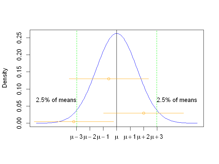
What proportion of such intervals would we expect to contain the true value \(\mu\)? Have a think about it and then click the button to the right.
From the plot above we can see that if we created intervals for each sample mean by stretching a distance of 1.96 standard errors in either direction then most of such intervals would cross the true value \(\mu\).
For the 2.5% of sample means that lie to the right of the right-hand dashed green line (which is at 1.96 standard errors above the mean), these intervals will miss the true value \(\mu\).
For the 2.5% of sample means that lie to the left of the left-hand dashed green line (which is at 1.96 standard errors above the mean), these intervals will miss the true value \(\mu\).
Thus, 95% of the intervals constructed in such a way will include the true value \(\mu\).
These intervals are called 95% confidence intervals.